# The Bellman Equation for Prediction Markets: How to Price Every Open Position You Hold
**作者**: Phosphen
**日期**: 2026-04-18T17:42:55.000Z
**来源**: [https://x.com/phosphenq/status/2045558709556744474](https://x.com/phosphenq/status/2045558709556744474)
---
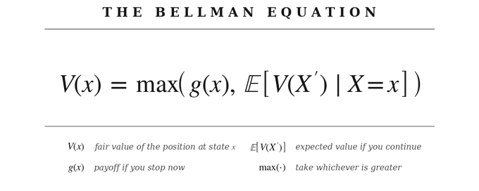
> One equation, four games, three centuries of math. Most traders never write it down. That's your edge.
There is a kind of trader who is right about events and still loses money.
Forecasts are accurate. Models are well-calibrated. The edge, measured in expected value, is real.
And she still underperforms a simpler trader who knows when to stop.
This is about why.
The math is older than prediction markets, older than Black-Scholes, older than modern portfolio theory. Richard Bellman formalized it in 1957, but the core was already embedded in a 1913 paper by Ernst Zermelo on chess. In prediction markets it turns out to be the single most consequential equation for actual PnL:

Every open position you hold on Polymarket is an instance of it. Most traders never write it down. That's the structural edge we're going to unpack.
What follows is a full, verified walkthrough. Four classical specializations of the equation, two of them solvable in 12 lines of Python, a worked end-to-end example on a synthetic prediction-market position, and a set of concrete rules you can apply to an open book tonight. Every formula has been fact-checked. Every number below was either derived on paper or computed with the solver alongside this piece.
## 1. Your open position is an optimal stopping problem
A Polymarket YES share pays $1 if the event resolves YES, $0 if NO. That's a European-payoff binary contract: the payoff rule is fixed at resolution date T.
But you can trade it continuously until T. At any moment you can hit the bid and walk away with the current market price M_t. You can also hold and face whatever market price or terminal payoff comes next.
Your position is therefore not a simple bet. It's a bet wrapped in a stopping problem.
The stopping problem looks like this. Let your private model estimate the probability of YES at time t as p_t. Define the continuation value V_t as the maximum of two things:
- Stop now: receive M_t.
- Continue: receive the expected value of Vt+1 under your model.
This is the Bellman recursion. The object V_t is called the Snell envelope of the reward process in the stopping-theory literature: the smallest supermartingale that dominates the stop payoff. It's the unique fair value of your position given your model.
Your trading edge comes from two things and only two things:
Information edge: your p_t is closer to the true probability than the market's.
Stopping edge: you solve the Bellman recursion and the market solves it badly.
The first is forecasting. The second is what this article is about. It's the one that scales with math.
## 2. Argentina bonds → a decoder for prices as probabilities
The first specialization. Imagine you have US Treasury forward rates iUSF and Argentine dollar-bond forwards iARGF. Both priced in dollars, both trade in the same market, both risk-free in everything except default. No-arbitrage forces the forward gap to encode the default probability exactly:

Derivation: a US zero has PV = 1/(1+i_US). An Argentine zero pays $1 with probability (1 − d) and $0 on default, so its PV is (1 − d)/(1 + i_US). Setting that equal to the observed price 1/(1 + i_ARG) and solving gives the formula above.
Worked example:
- US 1y forward: 4.2%
- ARG 1y forward: 12.8%
- 1 − d = 1.042 / 1.128 = 0.9238
- d ≈ 7.62% implied 1y default probability
First-order approximation when rates and defaults are small:

Spread IS probability. This is the entire content of the "credit spread" concept in fixed income.
Why a prediction-market trader cares.
A YES price of $0.67 on a binary market IS the market's risk-neutral probability of YES resolution. Every pair of correlated markets on Polymarket carries a default-probability structure relative to the other. Think "Trump wins" vs. "GOP takes popular vote", or "BTC ≥ $100k by Dec" vs. "BTC ≥ $120k by Dec".
When two such markets disagree in a way that can't be reconciled by any joint distribution, one of them is mispricing. You find these by computing the implied joint and comparing to what an arbitrage-free joint would require. Most traders never do this computation. Polymarket's basis inefficiencies are where a lot of the pure-arbitrage money has historically come from.
## 3. Zermelo 1913 → every finite game has a fair value
Second specialization. Ernst Zermelo proved in 1913 that chess has an optimal strategy, simply because it has a finite game tree. Every terminal position has a known value. By induction, every internal node has a value too:

You solve leaves first, propagate up, and the root has a unique value regardless of opponent strategy (under perfect play). Claude Shannon extended this in 1950 to depth-limited search with a positional evaluation function at the truncation boundary. This is the direct ancestor of how Stockfish computes moves today, and a structural cousin of what AlphaZero does with a neural evaluator.
Why a prediction-market trader cares.
Any position with a finite resolution horizon has a computable fair value, conditional on a specification of the transition dynamics. The tree is bigger than chess but not structurally different. Your edge is not "intuition." It's that your evaluation function at the pseudo-terminal nodes, where you stop computing and plug in an estimate, is better than the market's.
The region in (time, price) space where you choose to hold rather than stop is called the continuation region. Its boundary, the curve separating "hold" from "stop", is a free boundary. Solving the Bellman recursion is equivalent to finding that free boundary. That connection between optimal stopping and free boundary problems is why techniques from partial differential equations apply directly to trading problems in the continuous-time limit.
## 4. The red-black game → the option to stop has measurable value
Third specialization, this one quantitative. 52-card deck. 26 red, 26 black. Draw one at a time. Black pays +$1, red pays −$1. Quit whenever.
Naive analysis: expected value of a draw is zero. Skip it.
Actual optimal value: V(26, 26) = $2.6245.
The $2.6245 isn't coming from the cards. It's coming from the option to stop. Your downside is bounded below by zero (you can always play to the end of the deck, netting exactly zero). Your upside is not bounded (any favorable run lets you stop with a profit). Bounded downside plus unbounded upside plus the freedom to choose when to stop is a textbook free call option.
The Bellman recursion with g(x) = 0:

With boundaries V(0, R) = 0 and V(B, 0) = B. Solve in 12 lines of Python:
This is the simplest non-trivial optimal-stopping problem with a closed-form solver and immediate intuition. You should be able to derive it from scratch on a whiteboard. If you can, you understand optimal stopping.
## 5. The corollary most traders miss: the option is front-loaded
Here is where the lecture everyone cites on this problem gets truncated. The standard punch line is: "even when the deck is stacked against you, you should keep playing." Technically true. But the magnitudes tell a richer story. Run the solver at each state of a 5-black-run:
Yes, V(21, 26) is strictly positive, so optimal play says keep drawing. But it's $0.05. The option you held at the start was worth $2.62. After five favorable draws, 98% of the option's value has already been realized, not remaining. By the sixth black, the option is dead.
The real lesson.
The optionality in a stopping problem is front-loaded. Most of the value is captured in the first few decisions, not the last ones. A trader who enters early, at maximum uncertainty, holds the full option. A trader who chases a market after it has already drifted in the expected direction is buying what amounts to a deeply in-the-money position with almost no extrinsic value left. The edge is in early entry, not late conviction.
Polymarket translation.
A market at $0.50 on a binary event with 60 days to resolution has the most optionality. The same market at $0.85 with 5 days to resolution has almost none, regardless of how confident you are in YES. This is why "obvious" prediction-market positions pay so poorly: by the time it's obvious, the option has already been exercised by the tape.
## 6. The secretary problem → threshold decay
Fourth specialization. 1,000 candidates, each with i.i.d. Uniform(0, 1) suitability, sequential, no recall. The reward is the value of the accepted candidate. Reject all and your reward is zero.
Let V(t) be the value of optimal play with t candidates remaining. The recursion:

Simplify by expanding the second term: (1 − V(t−1)) · (1 + V(t−1))/2 = (1 − V(t−1)²) / 2. Add the first term V(t−1)² and you get:

Boundary: V(1) = 1/2 (you accept the last candidate unconditionally; her expected value is 1/2). The optimal threshold at step t is exactly V(t−1): accept the candidate iff her draw exceeds the value of all future play.
V(t) → 1 as t → ∞ (you're picking from an ocean). The convergence is slow: ε(t) ≈ 2/t + O(log t / t²), which means even at t = 1000 you're two-thousandths below the cap.
There's a famous near-identity. Asymptotically V(t) is close to (t − 1)/(t + 1), which is exactly the expected value of the second-highest order statistic of t uniform draws on [0, 1]:

For N = 1000, V(1000) ≈ 0.99802 and (N − 1)/(N + 1) ≈ 0.99800. They differ in the fifth decimal place. The poetic interpretation: on average, you end up with the second-best candidate you'd have seen. There is always one other person you regret not waiting for. The regret is baked into the math.
Polymarket translation.
Every Polymarket market has an implicit "secretary problem" structure because of the resolution countdown. Your reservation price, the price at which you'd sell, must decay as T approaches, for the same mathematical reason V(t) grows: the continuation value of waiting shrinks as the number of future states shrinks. A trader who uses a flat reservation price ("I sell at 60 cents") is throwing away PnL on every trade, because the fair threshold changes every day. The optimal rule is dynamic and computable.
## 7. Multiple stopping → scaling out is mathematically optimal
The single-stop problem is the first layer. In practice, a size-$50k position on a thin Polymarket book cannot be exited in one click without visible slippage. You scale out.
Kobylanski, Quenez, and Rouy-Mironescu (arXiv 0910.2788, published 2009) formalized the d-stop problem. Pick d stopping times τ1 < τ2 < … < τd and collect a reward:

Their main result is a reduction principle. The d-stop value function is the single-stop value of a transformed problem whose payoff is built from the (d − 1)-stop value:

In words: solve the 1-stop problem for the last clip, then recurse backward, each layer's reward being the next layer's expected continuation value. The d-stop value is strictly larger than d copies of the 1-stop value, because later clips benefit from information revealed by earlier ones.
Trading implication.
Scaling out of a Polymarket position in three clips at graduated prices dominates a one-shot exit in EV terms, provided the transitions are nontrivial. Each clip is its own stopping problem, conditioned on the history of previous clips. This is the formal justification for "laddering" exits that experienced traders already do by feel. The math says they're right.
## 8. A Polymarket worked example, end-to-end
Position: you hold 10,000 YES shares of a binary market. Cost basis $0.38. Current market $0.52. Your calibrated model says true resolution probability is 0.60. 60 days to resolution.
Step 1. Terminal values at resolution date T.
- VT(YES) = $1.00
- VT(NO) = $0.00
Step 2. Expected value at t = 0 under your model.
- V0 = 0.60 · 1.00 + 0.40 · 0.00 = $0.60
Step 3. Compare to market.
- Market $0.52 < V0 $0.60 → your fair value is above market → buy more.
Step 4. Exit rule with threshold decay.
- Flat rule: "sell at 0.65", greedy and ignores remaining time.
- Decaying rule: sell when market first hits a time-discounted fair value:

- At T, the threshold collapses to zero and the market decides for you.
Step 5. Multiple stopping for the 10k shares.
Split into three clips of roughly 3,300 shares each.
- Clip 1: exit when market first touches 0.56
- Clip 2: exit when market first touches 0.60
- Clip 3: hold to resolution or to 0.65, whichever first
Step 6. Simulate.
Average exit ~$0.60. Cost basis $0.38. Expected PnL per share ~$0.22. On 10,000 shares: ~$2,200 expected PnL. The forecasting edge (true 0.60 vs market 0.52) is what creates the money. Backward induction and multi-clip exits are what let you realize it consistently instead of path-by-path.
Note the asymmetry: 60% of paths resolve YES, and on those your last clip reaches $1.00, but 40% resolve NO and the last clip is $0. The averaging across clips is what extracts the expected value of your edge while capping path-dependent variance. This is the Kobylanski result made real.
## 9. Seven rules
Write the Bellman. V = max(stop, continue). Every open position is an instance.
Solve terminals first. Resolution payoffs are known; everything else is induction backward.
Spread is probability. Gaps between correlated market prices encode joint-distribution information.
The option is front-loaded. Early entry at maximum uncertainty captures the most optionality. Late entry after drift captures almost none.
Threshold must decay. Flat reservation prices leak money because the continuation value changes every day.
Scale out. d-stop beats 1-stop by a non-trivial margin whenever transitions are informative.
Forecasting is half the job. Stopping is the other half. Most traders treat it as an afterthought. Don't.
## Closing
Prediction markets are, at the deepest level, machines for aggregating stopping decisions.
You're not betting on whether an event will happen. The market is already pricing that, thousands of times a second, and doing a reasonable job. What you're betting on is when you'll act relative to everyone else. Whose stopping rule is closer to the true Bellman value at each node of the tree.
This is why two traders holding the same position at the same price can have radically different outcomes over time. The alpha in prediction markets isn't usually in being right. It's in being right enough, at the right moment, with the discipline to stop when the math tells you to.
The Bellman equation doesn't tell you what will happen. It tells you what to do when you don't know what will happen. In a world that sells confident forecasts as a product, that distinction is the product most people don't realize they need.
A forecaster predicts the future. A trader prices the option to wait for it. Most people think these are the same job. They aren't. The first is a talent. The second is a craft, and the craft has an equation.
Read the equation. Write the solver. Run it on a position tonight. Then decide whether the thing the market is selling you (the right to hold, exit, or add) is priced above or below what you now know it's worth.
That is the whole edge. Everything else is decoration.
## 相关链接
- [Phosphen](https://x.com/phosphenq)
- [@phosphenq](https://x.com/phosphenq)
- [11K](https://x.com/phosphenq/status/2045558709556744474/analytics)
- [Upgrade to Premium](https://x.com/i/premium_sign_up)
- [1:42 AM · Apr 19, 2026](https://x.com/phosphenq/status/2045558709556744474)
- [11.8K Views](https://x.com/phosphenq/status/2045558709556744474/analytics)
- [View quotes](https://x.com/phosphenq/status/2045558709556744474/quotes)
---
*导出时间: 2026/4/19 10:58:14*
---
## 中文翻译
# 预测市场的贝尔曼方程:如何为你持有的每一个开放头寸定价
**作者**: Phosphen
**日期**: 2026-04-18T17:42:55.000Z
**来源**: [https://x.com/phosphenq/status/2045558709556744474](https://x.com/phosphenq/status/2045558709556744474)
---

> 一个方程,四种博弈,三个世纪的数学。大多数交易员从未把它写下来。这就是你的优势。
有一种交易员,即便预测对了事件,却依然亏钱。
预测是准确的。模型经过校准。以期望值衡量的优势是真实存在的。
但她的表现依然不如一个知道何时收手的更简单的交易员。
本文将解释原因。
这段数学历史比预测市场更悠久,比布莱克-舒尔斯公式更古老,比现代投资组合理论更早。理查德·贝尔曼于1957年将其形式化,但其核心早已蕴含于恩斯特·策梅洛1913年关于国际象棋的论文中。在预测市场中,它是实际盈亏唯一最重要的方程:

你在 Polymarket 上持有的每一个开放头寸都是它的一个实例。大多数交易员从未把它写下来。这就是我们要拆解的结构性优势。
接下来的内容是一份完整、经过验证的指南。其中包括该方程的四种经典特化形式,其中两种可以用 12 行 Python 代码求解,一个合成预测市场头寸的端到端实战示例,以及一套你今晚就可以应用于开放市场的具体规则。每个公式都经过核实。下面的每个数字要么是在纸上推导出来的,要么是使用随附的求解器计算出来的。
## 1. 你的开放头寸是一个最优停止问题
Polymarket 上的 YES 份额如果事件结算为 YES 则支付 1 美元,如果为 NO 则支付 0 美元。这是一种欧式期权收益二元合约:收益规则在结算日 T 是固定的。
但你可以持续交易直到 T。在任何时刻你都可以点击卖出价并带着当前市场价格 M_t 离场。你也可以继续持有,面对接下来出现的任何市场价格或最终收益。
因此,你的头寸不仅仅是一个简单的赌注。它是一个包裹在停止问题中的赌注。
停止问题如下所示。设你的私有模型在时间 t 估计 YES 的概率为 p_t。将继续持有价值 V_t 定义为以下两者中的最大值:
- 现在停止:获得 M_t。
- 继续持有:获得你的模型下 Vt+1 的期望值。
这就是贝尔曼递归。在停止理论文献中,对象 V_t 被称为奖励过程的斯内尔包络:支配停止收益的最小上鞅。它是给定你的模型下,你头寸的唯 一公平价值。
你的交易优势仅来自两件事:
信息优势:你的 p_t 比市场的 p_t 更接近真实概率。
停止优势:你求解了贝尔曼递归,而市场求解得很糟糕。
第一点是预测。第二点是本文的主题。这是可以用数学扩展的优势。
## 2. 阿根廷债券 → 将价格解码为概率
第一个特化。假设你有美国国债远期利率 iUSF 和阿根廷美元债券远期利率 iARG。两者都以美元计价,都在同一市场交易,除了违约外在其他方面都是无风险的。无套利原则迫使远期利差精确编码违约概率:

推导:美国零息国债的现值 PV = 1/(1+i_US)。阿根廷零息债券以概率 (1 − d) 支付 1 美元,违约时支付 0 美元,因此其 PV 为 (1 − d)/(1 + i_US)。将其等于观察到的价格 1/(1 + i_ARG) 并求解即得到上述公式。
实战示例:
- 美国 1 年期远期:4.2%
- 阿根廷 1 年期远期:12.8%
- 1 − d = 1.042 / 1.128 = 0.9238
- d ≈ 7.62% 隐含 1 年期违约概率
当利率和违约率较小时的一阶近似:

利差即概率。这就是固定收益中“信用利差”概念的全部内容。
为什么预测市场交易员要在意这个。
二元市场上 0.67 美元的 YES 价格就是市场对 YES 结算的风险中性概率。Polymarket 上每一对相关的市场相对于彼此都携带一个违约概率结构。想想“特朗普获胜”与“共和党赢得普选”,或者是“12 月 BTC ≥ $100k”与“12 月 BTC ≥ $120k”。
当两个这样的市场出现无法通过任何联合分布调和的分歧时,其中一个就是定价错误的。你可以通过计算隐含联合分布并将其与无套利联合分布所要求的值进行比较来发现这些。大多数交易员从不做这个计算。Polymarket 的基低效率历史上是许多纯套利资金的来源。
## 3. 策梅洛 1913 → 每一个有限博弈都有公平价值
第二个特化。恩斯特·策梅洛在 1913 年证明了国际象棋具有最优策略,仅仅因为它具有有限的博弈树。每个终端位置都有一个已知的价值。通过归纳法,每个内部节点也都有一个价值:

你先求解叶子节点,然后向上传播,无论对手策略如何(在完美博弈下),根节点都有唯一的价值。克劳德·香农在 1950 年将其扩展到深度受限的搜索,并在截断边界使用位置评估函数。这是 Stockfish 今天计算棋步的直接祖先,也是 AlphaZero 使用神经评估器所做工作的结构表亲。
为什么预测市场交易员要在意这个。
任何具有有限结算期限的头寸,在给定转移动态规范的情况下,都具有可计算的公平价值。这个树比国际象棋大,但在结构上没有不同。你的优势不是“直觉”。而是你在伪终端节点(你停止计算并插入估计值的地方)的评估函数比市场的更好。
你在(时间,价格)空间中选择持有而不是停止的区域称为继续区域。它的边界,即区分“持有”和“停止”的曲线,是一个自由边界。求解贝尔曼递归等价于找到那个自由边界。这种最优停止与自由边界问题之间的联系,就是为什么偏微分方程的技术直接适用于连续时间极限下的交易问题。
## 4. 红黑博弈 → 停止期权具有可衡量的价值
第三个特化,这个是定量的。52 张牌的牌堆。26 张红,26 张黑。每次抽一张。黑牌支付 +1 美元,红牌支付 −1 美元。随时可以退出。
朴素分析:抽牌的期望值为零。跳过它。
实际最优价值:V(26, 26) = $2.6245。
这 $2.6245 不是来自牌。它来自停止的期权。你的下行风险受到零的下限约束(你总是可以打完这副牌,净得恰好零)。你的上行空间没有限制(任何有利的运行都能让你带着利润停止)。有界的下行风险加上无界的上行空间,加上选择何时停止的自由,这就是教科书式的免费看涨期权。
带有 g(x) = 0 的贝尔曼递归:

边界为 V(0, R) = 0 和 V(B, 0) = B。用 12 行 Python 求解:
这是最简单的非平凡最优停止问题,具有闭式求解器和直观的直觉。你应该能够从零开始在白板上推导它。如果你能做到,你就理解了最优停止。
## 5. 大多数交易员遗漏的推论:期权是前置的
这就是每个人引用的关于这个问题的讲座被截断的地方。标准的结论是:“即使牌堆对你不利,你也应该继续玩。” 技术上是真的。但幅度讲述了一个更丰富的故事。在 5 次连续黑牌运行的每个状态下运行求解器:
是的,V(21, 26) 是严格正的,所以最优策略说继续抽牌。但它只有 $0.05。你开始时持有的期权价值 $2.62。在五次有利的抽取之后,期权价值的 98% 已经被实现,而不是剩余的。到了第六张黑牌,期权就死了。
真正的教训。
停止问题中的期权性是前置的。大部分价值是在最初的几个决策中捕获的,而不是最后的。一个在最大不确定性时尽早进入的交易员持有完整的期权。一个在市场已经向预期方向漂移后追逐市场的交易员,买入的是相当于深度价内且几乎没有剩余外在价值的头寸。优势在于早期进入,而不是后期信念。
Polymarket 翻译。
一个还有 60 天结算的二元事件市场,价格为 $0.50 时具有最多的期权性。同样的市场在还有 5 天结算、价格为 $0.85 时几乎没有期权性,无论你对 YES 有多大的信心。这就是为什么“明显”的预测市场头寸回报如此之低:当它变得明显时,期权已经被行情行使了。
## 6. 秘书问题 → 阈值衰减
第四个特化。1000 名候选人,每个人都有独立同分布的 Uniform(0, 1) 适用性,顺序进行,不可回溯。奖励是被接受候选人的价值。拒绝所有人,你的奖励为零。
设 V(t) 为剩余 t 名候选人时最优博弈的价值。递归关系:

通过展开第二项来简化:(1 − V(t−1)) · (1 + V(t−1))/2 = (1 − V(t−1)²) / 2。加上第一项 V(t−1)² 你得到:

边界:V(1) = 1/2(你无条件接受最后一个候选人;她的期望值是 1/2)。在步骤 t 的最优阈值恰好是 V(t−1):当且仅当她的抽取超过所有未来博弈的价值时接受该候选人。
当 t → ∞ 时,V(t) → 1(你是在海洋中挑选)。收敛速度很慢:ε(t) ≈ 2/t + O(log t / t²),这意味着即使在 t = 1000 时,你也只比上限低千分之二。
有一个著名的近似恒等式。渐近地,V(t) 接近 (t − 1)/(t + 1),这恰好是 [0, 1] 上 t 次均匀抽取的第二大顺序统计量的期望值:

对于 N = 1000,V(1000) ≈ 0.99802 且 (N − 1)/(N + 1) ≈ 0.99800。它们在第五位小数有所不同。诗意的解释是:平均而言,你最终得到的是你会见过的第二好的候选人。总有另一个人让你后悔没有等下去。这种遗憾被 baked in 到数学中。
Polymarket 翻译。
每个 Polymarket 市场都有一个隐含的“秘书问题”结构,因为有结算倒计时。你的保留价格,即你愿意出售的价格,必须随着 T 的逼近而衰减,原因与 V(t) 增长的数学原因相同:等待的继续价值随着未来状态数量的减少而减少。使用固定保留价格(“我以 60 美分卖出”)的交易员在每一笔交易上都在扔掉 PnL,因为公平阈值每天都在变化。最优规则是动态且可计算的。
## 7. 多重停止 → 分批平仓在数学上是最优的
单次停止问题是第一层。在实践中,在流动性不足的 Polymarket 订单簿上 5 万美元的头寸不可能在不产生明显滑点的情况下一键平仓。你会分批平仓。
Kobylanski、Quenez 和 Rouy-Mironescu(arXiv 0910.2788,发表于 2009 年)将 d-停止问题形式化。选取 d 个停止时间 τ1 < τ2 < … < τd 并收集奖励:

他们的主要结果是一个归约原则。d-停止价值函数是一个变换问题的单停止价值,该问题的收益由 (d − 1)-停止价值构成:

用语言来说:为最后一笔平仓求解 1-停止问题,然后向后递归,每一层的收益都是下一层的期望继续价值。d-停止价值严格大于 d 个 1-停止价值的副本,因为后面的平仓受益于前面平仓揭示的信息。
交易含义。
在三个批次中以阶梯价格平仓 Polymarket 头寸,在期望值上优于一次性退出,前提是转移是非平凡的。每一笔平仓都是它自己的停止问题,以先前平仓的历史为条件。这就是经验丰富的交易员凭直觉所做的“梯式”退出的形式化证明。数学说他们是对的。
## 8. 一个 Polymarket 实战示例,端到端
头寸:你持有二元市场的 10,000 股 YES 份额。成本基础 $0.38。当前市场 $0.52。你经过校准的模型说真实结算概率是 0.60。距离结算还有 60 天。
步骤 1. 结算日 T 的终端价值。
- VT(YES) = $1.00
- VT(NO) = $0.00
步骤 2. 你的模型下 t = 0 时的期望值。
- V0 = 0.60 · 1.00 + 0.40 · 0.00 = $0.60
步骤 3. 与市场比较。
- 市场 $0.52 < V0 $0.60 → 你的公平价值高于市场 → 买入更多。
步骤 4. 带有阈值衰减的退出规则。
- 固定规则:“在 0.65 卖出”,贪婪且忽略了剩余时间。
- 衰减规则:当市场首次触及时间折现后的公平价值时卖出:

- 在 T 时,阈值坍缩为零,市场替你做出决定。
步骤 5. 针对 1 万股的多重停止。
分成三批,每批约 3,300 股。
- 第 1 批:当市场首次触及 0.56 时退出
- 第 2 批:当市场首次触及 0.60 时退出
- 第 3 批:持有到结算或到 0.65,取先发生的那个
步骤 6. 模拟。
平均退出价 ~$0.60。成本基础 $0.38。每股期望 PnL ~$0.22。在 10,000 股上:~$2,200 期望 PnL。预测优势(真实 0.60 vs 市场 0.52)是创造资金的原因。反向归纳和多批次退出让你能够始终如一地实现它,而不是依赖于单一路径。
注意不对称性:60% 的路径结算为 YES,在这些路径上你的最后一批达到 $1.00,但 40% 结算为 NO,最后一批是 $0。跨批次的平均化提取了你的优势的期望值,同时限制了路径依赖的方差。这就是 Kobylanski 结果的现实体现。
## 9. 七条规则
写下贝尔曼方程。V = max(停止, 继续)。每个开放头寸都是一个实例。
先求解终端。结算收益是已知的;其他一切都是向后归纳。
利差即概率。相关市场价格之间的差距编码了联合分布信息。
期权是前置的。在最大不确定性时尽早进入能捕获最多的期权性。在漂移后晚点进入几乎捕获不到期权性。
阈值必须衰减。固定的保留价格会漏钱,因为继续价值每天都在变化。
分批平仓。只要转移能提供信息,d-停止就以非平凡的幅度优于 1-停止。
预测是一半的工作。停止是另一半。大多数交易员把停止当成事后诸葛亮。别这样。
## 结语
在最深的层面上,预测市场是聚合停止决策的机器。
你不是在赌事件是否会发生。市场已经对此定价,每秒数千次,并且做得相当不错。你赌的是相对于其他人你何时行动。谁的停止规则在树的每个节点上更接近真实的贝尔曼价值。
这就是为什么两个以相同价格持有相同头寸的交易员随着时间的推移可能会有截然不同的结果。预测市场中的 Alpha 通常不在于“对”。而在于在正确的时刻足够“对”,并有在数学告诉你停止时停止的纪律。
贝尔曼方程不告诉你会发生什么。它告诉你当你不知道会发生什么时该怎么做。在一个自信预测被当作产品推销的世界里,这种区别是大多数人没意识到的他们需要的产品。
预测者预测未来。交易员为等待未来的期权定价。大多数人认为这是同一份工作。它们不是。第一份是天赋。第二份是手艺,而这门手艺有一个方程。
读懂方程。编写求解器。今晚在一个头寸上运行它。然后决定市场卖给你的东西(持有、退出或加仓的权利)的价格是高于还是低于你现在知道它的价值。
这就是全部的优势。其他一切都是装饰。