# How to Use Neural Networks to Win Every Trade Before It Even Starts
**作者**: Roan
**日期**: 2026-04-28T15:45:50.000Z
**来源**: [https://x.com/RohOnChain/status/2052043443766194272](https://x.com/RohOnChain/status/2052043443766194272)
---
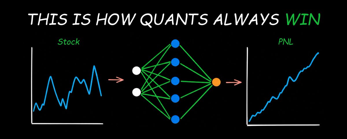
I am going to break down how hedge funds use neural networks to extract edge before the trade even happens & share the exact implementation framework you can build today.
Let's get straight to it.
> Bookmark This -
> I'm Roan, a backend developer working on system design, HFT-style execution, and quantitative trading systems. My work focuses on how prediction markets actually behave under load. For any suggestions, thoughtful collaborations, partnerships DMs are open.
The way most traders lose money has nothing to do with their market thesis.
They are right about direction more often than they think. The problem is they are operating on one signal, one indicator, one gut feeling. They are making probability decisions without a probability framework. And markets punish that mistake reliably and repeatedly.
Neural networks solve a fundamentally different problem. They do not predict the future. What they do is learn the expectation function hidden inside historical data. The mathematical relationship between what you can observe right now and what the market is statistically most likely to do next. And they do this across thousands of variables simultaneously in ways no human eye can see and no single indicator can capture.
The largest funds already know this. Two Sigma runs over 10,000 live signals through machine learning models simultaneously. Citadel's quantitative research division deploys deep learning architectures across equity, options, and macro strategies. Renaissance Technologies built the Medallion Fund entirely on this framework decades before anyone else understood what they were doing. The fund returned 66 percent annually before fees over 30 years. That is not luck. That is the systematic application of statistical learning at scale.
The entry level quant researcher building these models at those firms earns between $350,000 and $650,000 in total compensation. Not because the job is glamorous. Because finding a reliable edge in financial data using mathematics is genuinely one of the hardest unsolved problems in applied science.
If you have not yet read the complete quant roadmap covering the mathematical foundation underneath everything in this article, start there first.
> **Roan@RohOnChain**: [原文链接](https://x.com/RohOnChain/status/2049153122027900948)
>
AI and machine learning hiring in quantitative finance accelerated sharply through 2025. Every major systematic fund is building signal generation infrastructure powered by deep learning. And yet most traders who try to implement neural networks into their strategy fail at the same predictable step for the same predictable reason.
This article tells you exactly what that step is and exactly how to avoid it. Then it gives you the complete implementation framework from data preparation through live signal deployment.
By the end of this article you will understand exactly how neural networks learn from data and what they are actually computing when they make a prediction, why applying them directly to price charts is guaranteed to fail and what the correct input is, which architecture works best for sequential market data and why, the complete rigorous training framework that separates real edge from self-deception and the full implementation pipeline to deploy your first neural network trading signal.
Note: This article is deliberately long. Every part builds on the one before it. If you are serious about adding a genuine quantitative edge to your trading, read every single word. If you are looking for a shortcut, this is not for you.
## Part 1: What a Neural Network Actually Computes
Before you build anything, you need to understand what is actually happening when a neural network trains on data. Most explanations skip this and go straight to code. That is why most implementations fail.
A neural network is a parameterized composite function. You give it a vector of inputs. It applies a sequence of linear transformations interleaved with non-linear activation functions. It produces an output. The formal structure is:
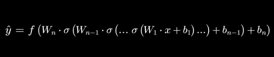
Where W_i are weight matrices, b_i are bias vectors, and σ is a non-linear activation function applied element-wise. This is the mathematical reality underneath every neural network regardless of how it is visualized.
The power is in training. You have a dataset of input-output pairs. The network starts with random parameters. It makes a prediction. It computes the error between that prediction and the actual observed output. It adjusts the parameters in the direction that reduces the error. It repeats this millions of times.
The formal objective is minimizing a loss function. For regression tasks the standard choice is mean squared error:
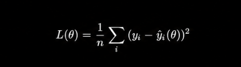
Where θ represents all learnable parameters, yᵢ is the actual observed value, and ŷᵢ is the model prediction. The optimization proceeds by computing the gradient of the loss with respect to the parameters and taking a step in the negative gradient direction: θ ← θ - α · ∇_θ L(θ)
Where α is the learning rate. This is stochastic gradient descent. Every modern deep learning optimizer is a variation of this with adaptive step sizes, momentum terms, or second-order approximations layered on top.
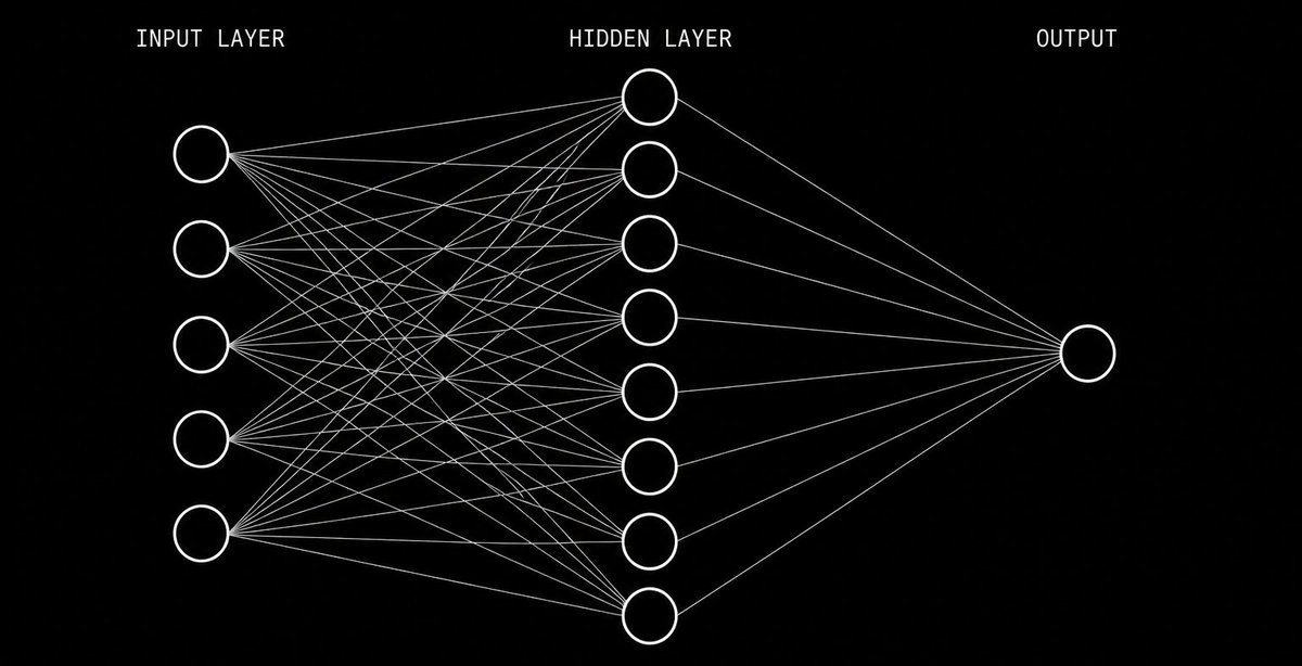
A feedforward neural network passes inputs through weighted layers to produce an output that approximates the conditional expectation of the target variable.
Now here is the insight that changes how you interpret everything a neural network produces.
When you train a network to minimize squared error against a target variable, what does it learn? It learns the conditional expectation of that variable given your inputs. The function that minimizes E[(Y - f(X))²] is exactly E[Y|X]. This is not a prediction in the colloquial sense. It is a mathematical expectation. The weighted average outcome across all scenarios consistent with the observed inputs.
The proof of this is straightforward. Expand the squared loss:
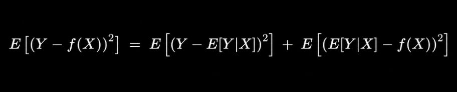
The first term is irreducible variance. The second term is minimized by setting f(X) = E[Y|X]. The optimal predictor under squared error is the conditional mean.
This has a profound practical implication. When you roll a fair die 10,000 times and train a neural network to minimize squared error against the outcomes, it will predict 3.5. Can a die land on 3.5? No. But 3.5 is the value that minimizes the expected squared error. The network is computing the expectation, not the next realization.
Why does neural networks specifically outperform simpler models at learning this conditional expectation? The universal approximation theorem. A feedforward network with a single hidden layer containing sufficient neurons can approximate any continuous function on a compact subset of Rⁿ to arbitrary precision. For deep networks with multiple layers, the approximation becomes exponentially more efficient in terms of the number of parameters required.
This means: if there is any smooth mathematical relationship between your input features and your target variable, a properly architected neural network can find it. The question is never whether the network can learn the function. The question is whether the function you want it to learn is actually stable enough across time to be worth learning.
## Part 2: Why Price Prediction Fails and What to Do Instead
This is the most important section in the article. The mistake described here is made by virtually every trader who tries to implement neural networks for the first time. Understanding why it fails is the prerequisite for everything that works.
The failure mode is this: take 500 days of closing prices, feed them into an LSTM, ask it to predict day 501.
In-sample, the predictions look smooth and close to actual prices. Out-of-sample, the model predicts something roughly constant or reverts to a recent mean while prices move somewhere completely different. The model appears to have learned nothing useful.
This is not a model failure. It is a data distribution failure.
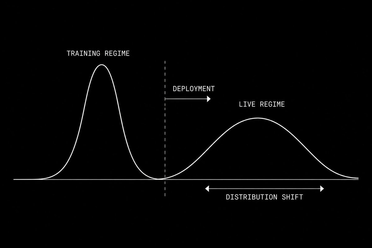
The distribution governing market returns shifts continuously over time. A model trained on the left regime learns the wrong expectation function for the right regime.
Recall from Part 1: a neural network learns E[Y|X], the conditional expectation of Y given X. This expectation is only meaningful if the data generating distribution P(Y|X) is stable over time. If that distribution shifts, the conditional expectation the model learned from historical data no longer describes the expectation in the present.
Formally, this is the problem of non-stationarity. A time series {Xₜ} is stationary if its joint distribution P(Xₜ₁, Xₜ₂, ..., Xₜₙ) is invariant to time shifts. Financial price series are non-stationary in the strongest possible sense. The distribution governing equity returns in 2008 is structurally different from the distribution governing them in 2021. Mean, variance, autocorrelation, and tail behavior all shift as a function of regime, liquidity, volatility clustering, and macro conditions.
The consequence is visible in any backtest of a price-predicting neural network. The model trained on 2015 to 2019 data learns the expectation structure of that regime. When the distribution shifts in 2020, the model is fitting a moving target. Its predictions are always wrong in a systematic way that reveals it is modeling the past distribution, not the present one.
What is the solution?
Feature engineering to produce stationary or near-stationary inputs. The target variable itself should also be constructed to be approximately stationary.
For inputs, the features that have exhibited reasonable stationarity across market regimes include:
Log returns over multiple windows: r_t = ln(P_t / P_{t-k}) for k in {1, 5, 20}
Volatility ratios: σ_short / σ_long where each σ is rolling realized volatility over different windows
Momentum signals normalized by volatility: r_t / σ_t, the return scaled by realized risk
Volume z-score: (V_t - μ_V) / σ_V computed over a rolling window
Spread-based signals: bid-ask spread relative to its historical distribution, or effective spread computed from trade price versus midpoint
Regime indicators: VWAP deviation, distance from rolling high and low, implied versus realized volatility ratio
For the target variable, instead of predicting next period price, predict next period direction as a binary classification problem: will the risk-adjusted return be positive? Or predict next period return z-scored against its recent distribution. Both targets are more stable than raw price or even raw return.
The practical test for whether a feature is useful: run an augmented Dickey-Fuller test on it. A p-value below 0.05 suggests the series is stationary. For features that fail this test, first-difference them or normalize by a rolling standard deviation.
Implementation note: In Python, this looks like:
```
from statsmodels.tsa.stattools import adfuller
import numpy as np
def check_stationarity(series, name):
result = adfuller(series.dropna())
print(f"{name}: ADF statistic={result[0]:.4f}, p-value={result[1]:.4f}")
return result[1] < 0.05
# Example feature engineering
returns = df['close'].pct_change()
vol_20 = returns.rolling(20).std()
vol_5 = returns.rolling(5).std()
features = {
'return_1d': returns,
'return_5d': df['close'].pct_change(5),
'vol_ratio': vol_5 / vol_20,
'momentum': returns / vol_20,
'volume_zscore': (df['volume'] - df['volume'].rolling(20).mean()) / df['volume'].rolling(20).std()
}
for name, series in features.items():
is_stationary = check_stationarity(series, name)
```
Every feature that fails the stationarity test is a feature that will cause your model to learn the wrong distribution.
## Part 3: The LSTM Architecture for Sequential Market Data
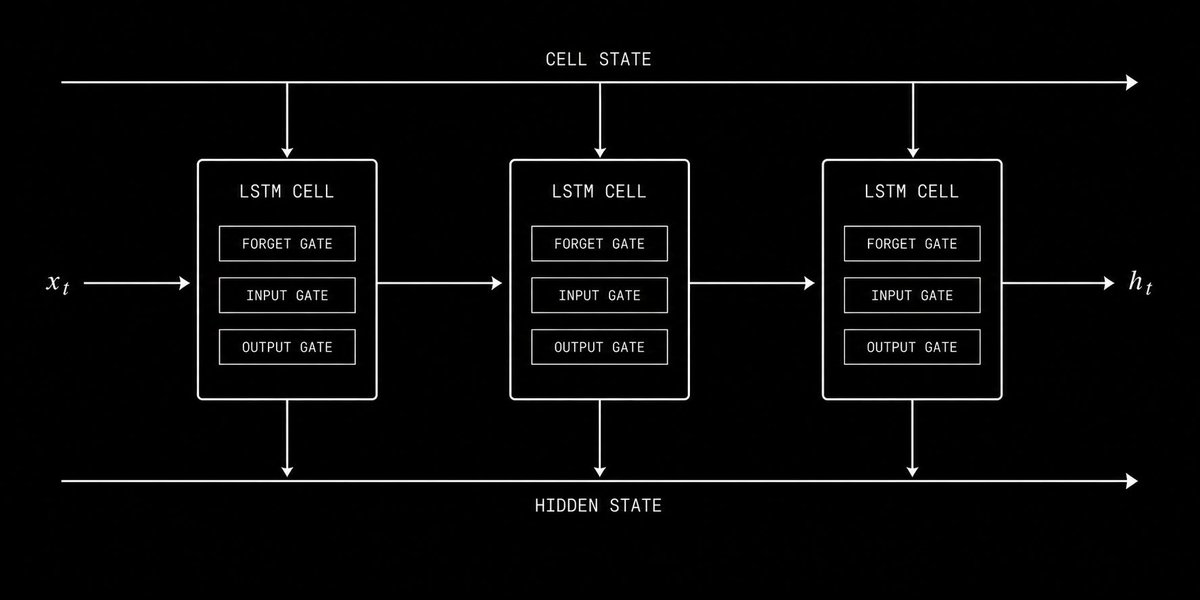
The LSTM forget gate, input gate, and output gate control what information persists across time steps, allowing the model to maintain context across weeks of market data.
Market data is sequential. The order of events carries information that a snapshot does not. What happened in the last five minutes is connected to what happens in the next five minutes through autocorrelation, momentum, mean reversion, and microstructure dynamics. The architecture you use must be capable of learning from this sequential structure.
A standard feedforward network treats every input independently. When you present it with day 100's feature vector, it has no knowledge of what days 1 through 99 looked like. For non-sequential data like the football throwing example from Part 1, this is fine. For time series data from financial markets, it throws away the most important information in your dataset.
The Recurrent Neural Network addresses this by passing a hidden state forward through time. At each time step t, the hidden state h_t is computed as:
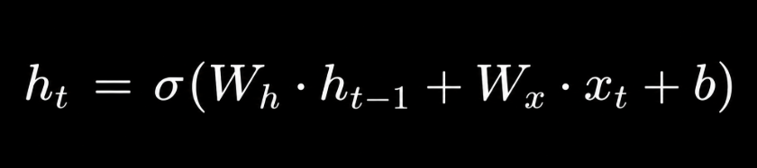
The hidden state encodes everything the network has learned from steps 1 through t-1 and combines it with the current input x_t. This is the memory mechanism. But basic RNNs suffer from the vanishing gradient problem: gradients diminish exponentially as they are backpropagated through time, making it effectively impossible to learn dependencies across more than a few time steps.
LSTM solves this with a gated memory architecture. Rather than a single hidden state, the LSTM maintains both a hidden state h_t and a cell state c_t. The cell state is the long-term memory. The hidden state is the working memory. Three learned gates control information flow:
Forget gate: f_t = σ(W_f · [h_{t-1}, x_t] + b_f) This gate decides what fraction of the previous cell state to discard. When markets transition between regimes, the forget gate allows the model to release outdated patterns and reset its understanding.
Input gate: i_t = σ(W_i · [h_{t-1}, x_t] + b_i), g_t = tanh(W_g · [h_{t-1}, x_t] + b_g) These gates decide what new information to write into the cell state.
Output gate: o_t = σ(W_o · [h_{t-1}, x_t] + b_o), h_t = o_t ⊙ tanh(c_t) This gate decides what to output from the cell state.
The cell state update combines forgetting and new writing: c_t = f_t ⊙ c_{t-1} + i_t ⊙ g_t
This architecture allows LSTM to maintain relevant context across sequences of 50, 100, or more time steps without the gradient vanishing problem. For daily trading strategies, this means the model can learn that a particular pattern of volatility compression three weeks ago predicts a specific type of breakout behavior today. No indicator-based system can capture relationships at that complexity.
Complete LSTM implementation in PyTorch:
```
import torch
import torch.nn as nn
import numpy as np
from sklearn.preprocessing import StandardScaler
class TradingLSTM(nn.Module):
def __init__(self, input_size, hidden_size=64, num_layers=2, dropout=0.2):
super(TradingLSTM, self).__init__()
self.hidden_size = hidden_size
self.num_layers = num_layers
self.lstm = nn.LSTM(
input_size=input_size,
hidden_size=hidden_size,
num_layers=num_layers,
dropout=dropout,
batch_first=True
)
self.dropout = nn.Dropout(dropout)
self.fc = nn.Linear(hidden_size, 1)
self.sigmoid = nn.Sigmoid()
def forward(self, x):
h0 = torch.zeros(self.num_layers, x.size(0), self.hidden_size)
c0 = torch.zeros(self.num_layers, x.size(0), self.hidden_size)
out, _ = self.lstm(x, (h0, c0))
out = self.dropout(out[:, -1, :])
out = self.fc(out)
return self.sigmoid(out)
def prepare_sequences(features, target, lookback=10):
X, y = [], []
for i in range(len(features) - lookback):
X.append(features[i:i+lookback])
y.append(target[i+lookback])
return np.array(X), np.array(y)
```
The lookback period is a critical hyperparameter. For daily strategies, start with a window of 10 to 20 trading days. For intraday strategies operating on 5-minute bars, a lookback of 24 periods covers two trading hours of context. The optimal lookback depends on the timescale of the patterns you are trying to capture and must be determined empirically through validation performance.
## Part 4: Training Without Fooling Yourself
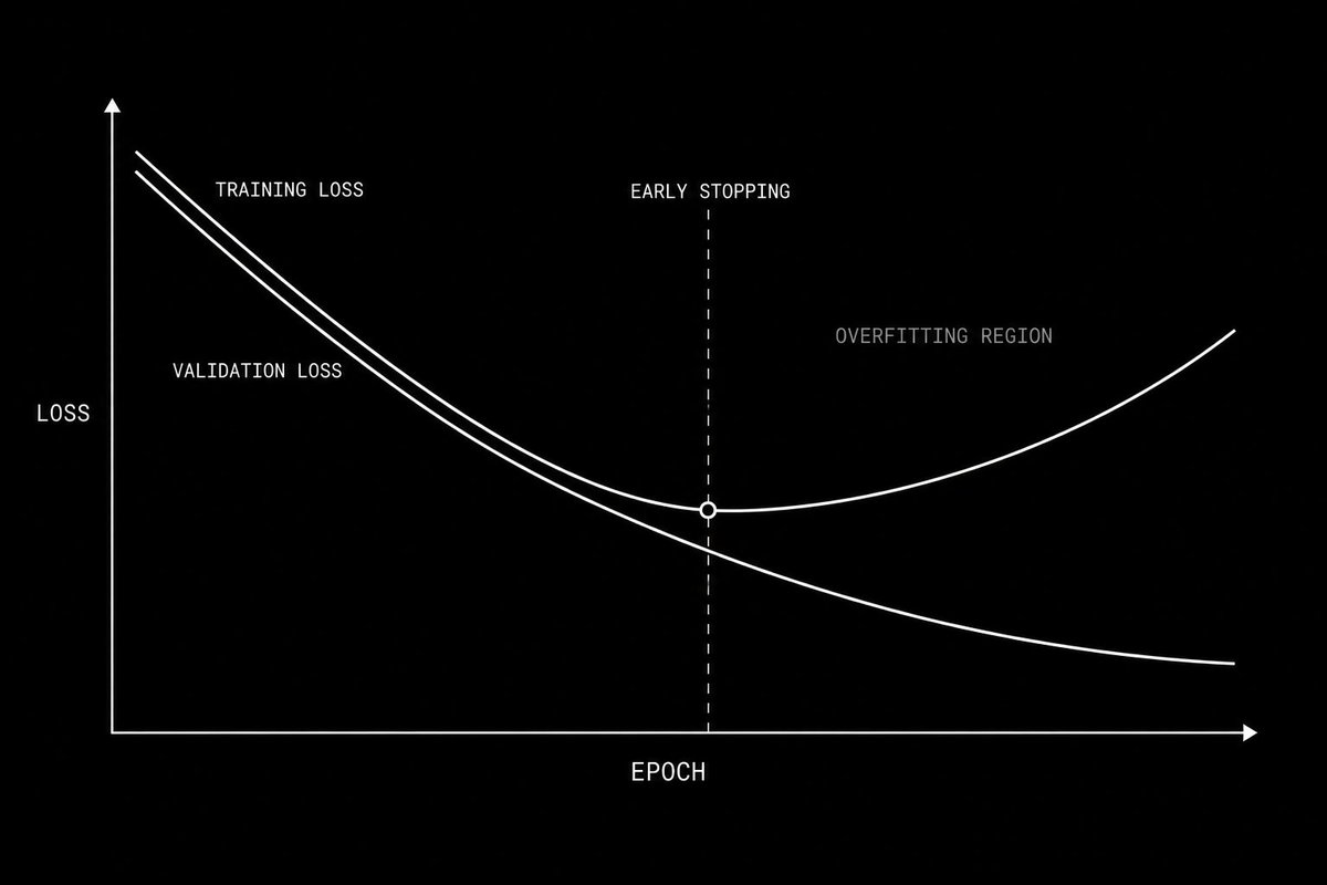
When training loss continues falling while validation loss rises, the model has crossed into overfitting. Early stopping saves the weights at the validation minimum.
Building the model is the easy part. The dangerous part is evaluating whether it actually learned something real versus memorizing the noise in your training data.
Overfitting is the central failure mode of machine learning in finance. An overfit model has found patterns in its training data that do not generalize. On training data it performs beautifully. On new data it performs at chance or worse. The critical problem is that overfit in-sample performance looks identical to genuine edge. You cannot distinguish them by looking at training metrics alone.
The solution is a rigorous three-way data split used in a specific sequential order.
The training set is where gradient descent runs. The model sees this data repeatedly during training and adjusts its parameters based on it. Never evaluate generalization performance on this set.
The validation set is data the model never trains on but that you monitor continuously during training. After each epoch, compute validation loss. The moment validation loss stops improving and begins increasing while training loss continues decreasing, you have found the overfitting threshold. Stop training immediately and save the model weights from the epoch with the lowest validation loss. This is early stopping and it is your primary defense against overfitting.
The test set is data the model has never influenced in any form. You use it exactly once: after all architecture decisions, all hyperparameter choices, and all feature engineering decisions have been finalized using the training and validation sets. The test set result is your honest estimate of live performance. Using the test set to make additional design decisions invalidates it.
For financial time series, these splits must be sequential. The training period comes first in time. The validation period follows. The test period is most recent. Randomizing the split would allow future information to contaminate training, a form of lookahead bias that guarantees your backtest looks better than live performance.
Complete training loop with early stopping:
```
def train_model(model, train_loader, val_loader, epochs=100, lr=0.001, patience=10):
optimizer = torch.optim.Adam(model.parameters(), lr=lr)
criterion = nn.BCELoss()
scheduler = torch.optim.lr_scheduler.ReduceLROnPlateau(
optimizer, patience=5, factor=0.5
)
best_val_loss = float('inf')
best_weights = None
patience_counter = 0
for epoch in range(epochs):
model.train()
train_loss = 0
for X_batch, y_batch in train_loader:
optimizer.zero_grad()
predictions = model(X_batch).squeeze()
loss = criterion(predictions, y_batch)
loss.backward()
torch.nn.utils.clip_grad_norm_(model.parameters(), max_norm=1.0)
optimizer.step()
train_loss += loss.item()
model.eval()
val_loss = 0
with torch.no_grad():
for X_batch, y_batch in val_loader:
predictions = model(X_batch).squeeze()
loss = criterion(predictions, y_batch)
val_loss += loss.item()
val_loss /= len(val_loader)
scheduler.step(val_loss)
if val_loss < best_val_loss:
best_val_loss = val_loss
best_weights = model.state_dict().copy()
patience_counter = 0
else:
patience_counter += 1
if patience_counter >= patience:
print(f"Early stopping at epoch {epoch}")
break
model.load_state_dict(best_weights)
return model
```
Gradient clipping is included in this implementation for a specific reason. LSTM gradients can explode during training when the learned sequences are long. Clipping the gradient norm to a maximum value of 1.0 prevents this without significantly affecting convergence speed.
The most rigorous evaluation framework for trading specifically is walk-forward validation. Rather than a single train-validation-test split, you roll a training window forward through time, train, test on the immediately following period, then advance the window and repeat. The concatenated out-of-sample predictions across all windows give you a realistic estimate of how the model would have performed if deployed live at each historical point.
Walk-forward validation:
```
def walk_forward_validation(features, target, train_size, test_size, step):
all_predictions = []
all_actuals = []
for start in range(0, len(features) - train_size - test_size, step):
train_end = start + train_size
test_end = train_end + test_size
X_train = features[start:train_end]
y_train = target[start:train_end]
X_test = features[train_end:test_end]
y_test = target[train_end:test_end]
scaler = StandardScaler()
X_train_scaled = scaler.fit_transform(X_train.reshape(-1, X_train.shape[-1]))
X_test_scaled = scaler.transform(X_test.reshape(-1, X_test.shape[-1]))
model = TradingLSTM(input_size=X_train.shape[-1])
# train model here
with torch.no_grad():
preds = model(torch.FloatTensor(X_test_scaled))
all_predictions.extend(preds.numpy())
all_actuals.extend(y_test)
return np.array(all_predictions), np.array(all_actuals)
```
The expected directional accuracy for a well-built model on good features is 52 to 57 percent. This sounds unremarkable. A 54 percent directional signal with a Sharpe ratio above 1.0, applied consistently across hundreds of trades with correct Kelly-derived position sizing, compounds into returns that outperform most discretionary traders over a multi-year horizon. The edge is in the consistency and the scale, not in the magnitude of any individual signal.
## Part 5: The Complete Implementation Pipeline and Deployment
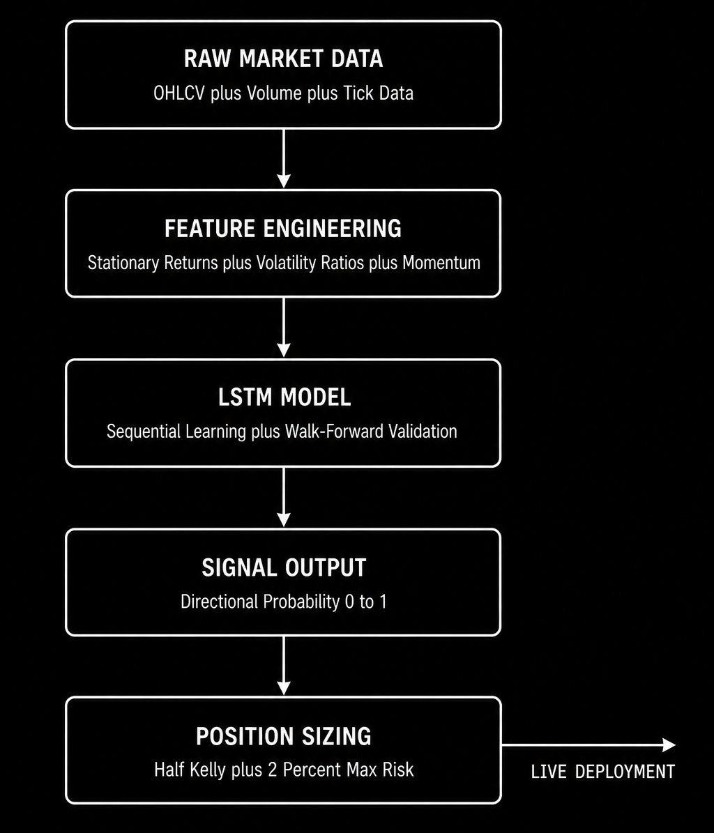
The end-to-end neural network trading signal pipeline from raw data to live position sizing.
This section takes everything from the previous four parts and assembles it into a production-ready signal pipeline. This is the complete end-to-end implementation.
Step 1: Data acquisition and cleaning
Use Polygondotio for institutional-grade tick and OHLCV data. For learning, yfinance is sufficient. Handle missing data, corporate actions, and splits before any feature engineering.
```
import yfinance as yf
import pandas as pd
ticker = yf.Ticker("SPY")
df = ticker.history(period="5y", interval="1d")
df = df[['Open', 'High', 'Low', 'Close', 'Volume']].copy()
df.dropna(inplace=True)
```
Step 2: Feature engineering
Build your complete stationary feature set. Every feature must pass the Augmented Dickey-Fuller test.
```
def build_features(df):
features = pd.DataFrame(index=df.index)
close = df['Close']
volume = df['Volume']
returns = close.pct_change()
features['return_1d'] = returns
features['return_5d'] = close.pct_change(5)
features['return_20d'] = close.pct_change(20)
vol_5 = returns.rolling(5).std()
vol_20 = returns.rolling(20).std()
features['vol_ratio'] = vol_5 / vol_20
features['momentum_norm'] = returns / vol_20
features['volume_zscore'] = (
(volume - volume.rolling(20).mean()) / volume.rolling(20).std()
)
high_low_range = (df['High'] - df['Low']) / close
features['range_norm'] = high_low_range / high_low_range.rolling(20).mean()
sma_5 = close.rolling(5).mean()
sma_20 = close.rolling(20).mean()
features['sma_ratio'] = sma_5 / sma_20 - 1
target = (returns.shift(-1) > 0).astype(int)
features = features.dropna()
target = target.loc[features.index]
return features, target
```
Step 3: Sequential split and scaling
```
def prepare_data(features, target, lookback=10, train_ratio=0.6, val_ratio=0.2):
n = len(features)
train_end = int(n * train_ratio)
val_end = int(n * (train_ratio + val_ratio))
scaler = StandardScaler()
features_scaled = scaler.fit_transform(features[:train_end])
features_array = np.vstack([
features_scaled,
scaler.transform(features[train_end:val_end]),
scaler.transform(features[val_end:])
])
X, y = prepare_sequences(features_array, target.values, lookback)
X_train = torch.FloatTensor(X[:train_end - lookback])
y_train = torch.FloatTensor(y[:train_end - lookback])
X_val = torch.FloatTensor(X[train_end - lookback:val_end - lookback])
y_val = torch.FloatTensor(y[train_end - lookback:val_end - lookback])
X_test = torch.FloatTensor(X[val_end - lookback:])
y_test = torch.FloatTensor(y[val_end - lookback:])
return X_train, y_train, X_val, y_val, X_test, y_test, scaler
```
Step 4: Model evaluation
Beyond directional accuracy, evaluate your model using metrics that matter for trading.
```
from sklearn.metrics import accuracy_score, roc_auc_score
import pandas as pd
def evaluate_trading_signal(predictions, actuals, returns):
pred_direction = (predictions > 0.5).astype(int)
accuracy = accuracy_score(actuals, pred_direction)
auc = roc_auc_score(actuals, predictions)
signal = np.where(pred_direction == 1, 1, -1)
strategy_returns = signal * returns
sharpe = strategy_returns.mean() / strategy_returns.std() * np.sqrt(252)
cumulative = (1 + strategy_returns).cumprod()
rolling_max = cumulative.cummax()
drawdown = (cumulative - rolling_max) / rolling_max
max_drawdown = drawdown.min()
print(f"Directional Accuracy: {accuracy:.4f}")
print(f"AUC-ROC: {auc:.4f}")
print(f"Annualized Sharpe: {sharpe:.4f}")
print(f"Maximum Drawdown: {max_drawdown:.4f}")
return accuracy, sharpe, max_drawdown
```
Step 5: Signal to position sizing
A neural network signal alone is not a trading strategy. You need position sizing. The Kelly fraction translates your model's edge into an optimal bet size:
> f* = (p × b - q) / b
Where p is your directional accuracy, q = 1 - p, and b is the average win-to-loss ratio. In practice, use half Kelly to account for parameter estimation error. Never risk more than 2 percent of capital on a single signal regardless of what Kelly recommends.
Step 6: Continuous monitoring and retraining
A model trained on historical data begins degrading the moment it is deployed. Market regimes shift. The conditional expectation the model learned becomes a progressively worse approximation of the current expectation. You must implement a monitoring system that tracks live performance against your validation baseline and triggers retraining when the distribution has shifted beyond an acceptable threshold.
The standard metric is the Kolmogorov-Smirnov statistic comparing your recent live prediction distribution to the historical validation distribution. When the KS statistic exceeds 0.1, retrain on the most recent data and re-evaluate before continuing to deploy.
For prediction markets and crypto specifically, regime shifts are more frequent and more violent than in equity markets. Retraining on a rolling 90-day window with walk-forward re-evaluation every 30 days is a reasonable baseline.
## The Summary
Neural networks do not give you a crystal ball. What they give you is a systematic, mathematically rigorous framework for extracting the conditional expectation of market behavior from historical data. When the features are stationary, the architecture is appropriate for sequential data, the training is disciplined and validated correctly, and the signal is sized with proper position management, the result is an edge that is consistent, scalable, and reproducible.
Two Sigma runs 10,000 signals simultaneously through this framework. Renaissance built the highest returning fund in financial history on it. The entry level researcher implementing it earns $650,000 per year.
The complete implementation is in this article. The mathematics is learnable. The code is buildable in a weekend. The only thing that separates the systematic funds from everyone else is knowing the correct framework and the discipline to follow it without cutting corners.
Now you know the framework.
Here is the question I want you to sit with.
A neural network trained on your current indicator set will learn the conditional expectation of market returns given those indicators. But the conditional expectation is only as good as the features you condition on. If you had to add exactly one new feature to your model that you believe no other systematic trader is using, what would it be and why?
Drop your answer in the comments.
There is no wrong answer but there are very revealing ones.
## 相关链接
- [Roan](https://x.com/RohOnChain)
- [@RohOnChain](https://x.com/RohOnChain)
- [Apr 28](https://x.com/RohOnChain/status/2049153122027900948)
- [1.7M](https://x.com/RohOnChain/status/2049153122027900948/analytics)
- [Upgrade to Premium](https://x.com/i/premium_sign_up)
- [11:10 PM · May 6, 2026](https://x.com/RohOnChain/status/2052043443766194272)
- [3,020 Views](https://x.com/RohOnChain/status/2052043443766194272/analytics)
- [View quotes](https://x.com/RohOnChain/status/2052043443766194272/quotes)
---
*导出时间: 2026/5/7 00:04:33*
---
## 中文翻译
# 如何利用神经网络在交易开始前锁定胜局
**作者**: Roan
**日期**: 2026-04-28T15:45:50.000Z
**来源**: [https://x.com/RohOnChain/status/2052043443766194272](https://x.com/RohOnChain/status/2052043443766194272)
---

我将深入剖析对冲基金如何利用神经网络在交易发生之前提取超额收益,并分享一个你今天就可以构建的精确实施框架。
直奔主题。
> 收藏本文 -
> 我是 Roan,一名后端开发者,专注于系统设计、高频交易(HFT)风格的执行以及量化交易系统。我的研究重点是预测市场在真实负载下的实际表现。欢迎通过私信提出任何建议、深入的合作或伙伴关系。
大多数交易者亏钱的原因与他们的市场逻辑无关。
他们判断正确的次数比他们想象的要多。问题在于他们仅依赖单一信号、单一指标或单纯的感觉。他们在没有概率框架的情况下做概率决策。而市场会反复而可靠地惩罚这种错误。
神经网络解决的是一个根本性的不同问题。它们并不预测未来。它们所做的是从历史数据中学习隐藏的期望函数。即你当前所能观察到的变量与市场接下来在统计上最可能的行为之间的数学关系。而且它们是同时针对数千个变量进行这种计算的,其方式是人眼无法察觉、任何单一指标也无法捕捉的。
最大的基金早已深知这一点。Two Sigma 通过机器学习模型同时运行超过 10,000 个实时信号。Citadel(城堡)的量化研究部门在股票、期权和宏观策略中部署了深度学习架构。Renaissance Technologies(文艺复兴科技)早在其他人理解他们在做什么之前的几十年里,就完全基于此框架建立了大奖章基金。该基金在 30 年内费前年化回报率为 66%。这并非运气。这是统计学习在大规模上的系统性应用。
在这些公司构建此类模型的初级量化研究员,总薪酬在 35 万美元到 65 万美元之间。这并不是因为工作光鲜亮丽。而是因为利用数学在金融数据中寻找可靠的优势,确实是应用科学中最难解决的未解难题之一。
如果你还没有阅读涵盖本文所有数学基础的完整量化路线图,请先从这里开始。
> **Roan@RohOnChain**: [原文链接](https://x.com/RohOnChain/status/2049153122027900948)
到 2025 年,量化金融领域的 AI 和机器学习招聘急剧加速。每个主要的系统性基金都在建立由深度学习驱动的信号生成基础设施。然而,大多数尝试将神经网络纳入其策略的交易者,都在同一个可预测的步骤失败了,原因也如出一辙。
本文将确切地告诉你那一步是什么,以及确切地如何避免它。然后,它将为你提供从数据准备到实时信号部署的完整实施框架。
读完本文后,你将准确理解:神经网络如何从数据中学习,以及它们在进行预测时实际计算的是什么;为什么将它们直接应用于价格图表注定会失败,正确的输入是什么;哪种架构最适合连续的市场数据及其原因;区分真实优势与自我欺骗的完整严格训练框架;以及部署你的第一个神经网络交易信号的完整实施流程。
注意:本文特意写得很长。每一部分都建立在前一部分的基础之上。如果你认真考虑为你的交易增加真正的量化优势,请读完每一个字。如果你在寻找捷径,本文不适合你。
## 第一部分:神经网络实际计算的是什么
在构建任何东西之前,你需要了解当神经网络在数据上训练时实际发生了什么。大多数解释跳过了这一点,直接进入代码。这就是为什么大多数实施会失败。
神经网络是一个参数化的复合函数。你给它一个输入向量。它应用一系列线性变换,中间穿插非线性激活函数。它产生一个输出。其形式结构如下:

其中 W_i 是权重矩阵,b_i 是偏置向量,σ 是逐元素应用的非线性激活函数。这就是无论可视化效果如何,每个神经网络底层数学现实。
威力在于训练。你有一组输入-输出对数据集。网络从随机参数开始。它进行预测。它计算该预测与实际观测输出之间的误差。它沿着减少误差的方向调整参数。它重复这一过程数百万次。
形式上的目标是最小化损失函数。对于回归任务,标准选择是均方误差:

其中 θ 代表所有可学习参数,yᵢ 是实际观测值,ŷᵢ 是模型预测。优化过程通过计算损失相对于参数的梯度,并沿着负梯度方向迈出一步来进行:θ ← θ - α · ∇_θ L(θ)
其中 α 是学习率。这就是随机梯度下降。每一种现代深度学习优化器都是它的变体,只是在上面叠加了自适应步长、动量项或二阶近似。

前馈神经网络将输入通过加权层传递,产生一个输出,该输出近似于目标变量的条件期望。
这里有一个见解,它会改变你解释神经网络产生的所有结果的方式。
当你训练一个网络来最小化相对于目标变量的平方误差时,它学到了什么?它学到了该变量在给定你的输入情况下的条件期望。最小化 E[(Y - f(X))²] 的函数正是 E[Y|X]。这不是口语意义上的预测。这是一个数学期望。即与观测到的输入相一致的所有场景下的加权平均结果。
其证明很简单。展开平方损失:

第一项是不可约方差。第二项通过设定 f(X) = E[Y|X] 来最小化。在平方误差下的最优预测器是条件均值。
这具有深刻的实际意义。当你掷一个公平的骰子 10,000 次并训练一个神经网络来最小化相对于结果的平方误差时,它会预测 3.5。骰子能停在 3.5 上吗?不能。但 3.5 是最小化预期平方误差的值。网络计算的是期望,而不是下一个实现值。
为什么神经网络在学习这种条件期望方面特别优于更简单的模型?通用近似定理。具有单隐含层且包含足够神经元的前馈网络可以以任意精度逼近 Rⁿ 紧密子集上的任何连续函数。对于具有多层深度网络,在所需参数数量方面,逼近变得呈指数级地更高效。
这意味着:如果你的输入特征和目标变量之间存在任何平滑的数学关系,架构合理的神经网络就能找到它。问题从来不是网络能否学习该函数。问题是你希望它学习的函数是否在时间跨度上足够稳定,以至于值得学习。
## 第二部分:为什么价格预测会失败以及该怎么做
这是文章中最重要的部分。这里描述的错误几乎每一个尝试首次实现神经网络的交易者都会犯。理解为什么它是失败的前提是理解所有有效的方法。
失败模式如下:获取 500 天的收盘价,将它们输入 LSTM(长短期记忆网络),要求它预测第 501 天。
在样本内,预测看起来很平滑,接近实际价格。在样本外,模型预测出大致恒定的值或恢复到最近的均值,而价格却走向了完全不同的地方。模型似乎没有学到任何有用的东西。
这不是模型失败。这是数据分布失败。

支配市场回报的分布随时间不断变化。在左侧区域训练的模型学习了针对右侧区域的错误期望函数。
回顾第一部分:神经网络学习 E[Y|X],即给定 X 时 Y 的条件期望。只有当数据生成分布 P(Y|X) 随时间稳定时,这个期望才有意义。如果该分布发生偏移,模型从历史数据中学到的条件期望就不再描述当前的期望。
形式上,这是非平稳性问题。如果时间序列 {Xₜ} 的联合分布 P(Xₜ₁, Xₜ₂, ..., Xₜₙ) 对于时间平移是不变的,则它是平稳的。金融价格序列在最强烈的意义上是非平稳的。支配股票回报的分布在 2008 年与在 2021 年有结构性差异。均值、方差、自相关性和尾部行为都随着区域、流动性、波动率聚类和宏观条件的变化而变化。
这一后果在任何价格预测神经网络的回测中都可见一斑。在 2015 年至 2019 年数据上训练的模型学习了该区域的期望结构。当分布在 2020 年发生偏移时,模型就像在拟合一个移动的目标。它的预测总是以一种系统性的方式出错,这表明它在对过去的分布建模,而不是当前的分布。
解决方案是什么?
特征工程,以产生平稳或近似平稳的输入。目标变量本身也应构造成近似平稳的。
对于输入,在不同市场区域表现出合理平稳性的特征包括:
多窗口对数回报率:r_t = ln(P_t / P_{t-k}),其中 k 属于 {1, 5, 20}
波动率比率:σ_short / σ_long,其中每个 σ 是不同窗口上的滚动已实现波动率
经波动率标准化的动量信号:r_t / σ_t,由已实现风险缩放的回报率
成交量 z-score:(V_t - μ_V) / σ_V,在滚动窗口上计算
基于价差的信号:买卖价差相对于其历史分布,或根据交易价格与中点计算的有效价差
区域指标:VWAP(成交量加权平均价)偏离度,距离滚动高点和低点的距离,隐含波动率与已实现波动率之比
对于目标变量,与其预测下一期的价格,不如将下一期的方向作为二元分类问题来预测:风险调整后的回报率是否为正?或者预测下一期回报率相对于其最近分布的 z-score。这两个目标都比原始价格甚至原始回报率更稳定。
判断特征是否有用的实际测试:对其进行增强迪基-富勒 检验。p 值低于 0.05 表明该序列是平稳的。对于未通过此检验的特征,先对它们进行一阶差分或按滚动标准差进行归一化。
实施说明:在 Python 中,这看起来像:
```
from statsmodels.tsa.stattools import adfuller
import numpy as np
def check_stationarity(series, name):
result = adfuller(series.dropna())
print(f"{name}: ADF statistic={result[0]:.4f}, p-value={result[1]:.4f}")
return result[1] < 0.05
# 示例特征工程
returns = df['close'].pct_change()
vol_20 = returns.rolling(20).std()
vol_5 = returns.rolling(5).std()
features = {
'return_1d': returns,
'return_5d': df['close'].pct_change(5),
'vol_ratio': vol_5 / vol_20,
'momentum': returns / vol_20,
'volume_zscore': (df['volume'] - df['volume'].rolling(20).mean()) / df['volume'].rolling(20).std()
}
for name, series in features.items():
is_stationary = check_stationarity(series, name)
```
任何未通过平稳性检验的特征都会导致模型学习错误的分布。
## 第三部分:用于连续市场数据的 LSTM 架构

LSTM 的遗忘门、输入门和输出门控制着哪些信息在不同时间步之间持续存在,允许模型在数周的市场数据中保持上下文。
市场数据是连续的。事件的顺序承载了快照所没有的信息。过去五分钟发生的事情通过自相关性、动量、均值回归和微观结构动力与接下来五分钟发生的事情相连。你使用的架构必须能够从这种连续结构中学习。
标准的前馈网络独立地处理每个输入。当你向它展示第 100 天的特征向量时,它不知道第 1 到第 99 天的样子。对于像第一部分中扔足球例子那样的非连续数据,这没问题。对于来自金融市场的时间序列数据,它丢弃了数据集中最重要的信息。
循环神经网络通过在时间上向前传递隐状态来解决这个问题。在每个时间步 t,隐状态 h_t 计算如下:

隐状态编码了网络从步骤 1 到 t-1 学到的所有内容,并将其与当前输入 x_t 结合。这就是记忆机制。但基本的 RNN 受梯度消失问题的困扰:梯度随时间反向传播呈指数级衰减,使得学习超过几个时间步的依赖关系实际上变得不可能。
LSTM 通过门控记忆架构解决了这个问题。LSTM 不仅维护一个隐状态 h_t,还维护一个单元状态 c_t。单元状态是长期记忆。隐状态是工作记忆。三个学习到的门控制信息流:
遗忘门:f_t = σ(W_f · [h_{t-1}, x_t] + b_f) 此门决定丢弃前一单元状态的多大部分。当市场在区域之间转换时,遗忘门允许模型释放过时的模式并重置其理解。
输入门:i_t = σ(W_i · [h_{t-1}, x_t] + b_i), g_t = tanh(W_g · [h_{t-1}, x_t] + b_g) 这些门决定将哪些新信息写入单元状态。
输出门:o_t = σ(W_o · [h_{t-1}, x_t] + b_o), h_t = o_t ⊙ tanh(c_t) 此门决定从单元状态输出什么。
单元状态更新结合了遗忘和新的写入:c_t = f_t ⊙ c_{t-1} + i_t ⊙ g_t
这种架构允许 LSTM 在 50、100 或更多时间步的序列中保持相关的上下文,而不会出现梯度消失问题。对于日常交易策略,这意味着模型可以学习到三周前特定的波动率压缩模式预测了今天特定类型的突破行为。没有任何基于指标的系统能捕捉到这种复杂度的关系。
PyTorch 中的完整 LSTM 实现:
```
import torch
import torch.nn as nn
import numpy as np
from sklearn.preprocessing import StandardScaler
class TradingLSTM(nn.Module):
def __init__(self, input_size, hidden_size=64, num_layers=2, dropout=0.2):
super(TradingLSTM, self).__init__()
self.hidden_size = hidden_size
self.num_layers = num_layers
self.lstm = nn.LSTM(
input_size=input_size,
hidden_size=hidden_size,
num_layers=num_layers,
dropout=dropout,
batch_first=True
)