PyTorch 训练流程速查表

✍ kozue🕐 2026-07-03📦 12.0 KB 🟢 已读 𝕏 文章列表

这是一份关于 PyTorch 训练流程的单页速查表。文章通过代码示例和原理解析，深入浅出地讲解了张量的核心概念、矩阵乘法、自动求导机制、反向传播以及梯度下降优化过程。同时涵盖了 `nn.Module` 常用组件如 Linear、ReLU 和 GELU 的使用，旨在帮助开发者快速理解深度学习引擎的运作原理。

PyTorch 深度学习教程张量 Autograd 机器学习速查表矩阵乘法反向传播 Python

# Your One-Page PyTorch Training Pipeline Cheat Sheet. **作者**: kozue **日期**: 2026-07-02T09:03:19.000Z **来源**: [https://x.com/0xkozue/status/2072607035624247732](https://x.com/0xkozue/status/2072607035624247732) --- 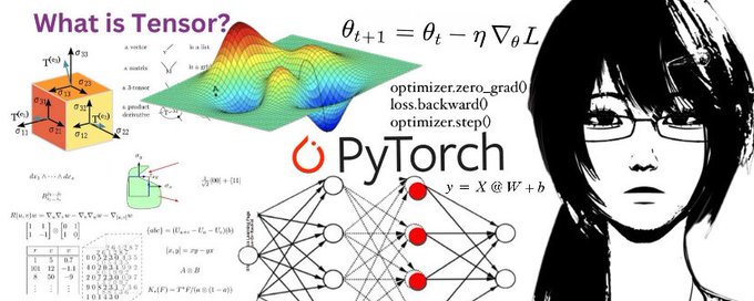![Image](/doc/2686/image/img_441ea20f0e06.jpg) > The entire engine of Deep Learning works by making tiny, continuous adjustments to a model's weights. This is my PyTorch training pipeline cheat sheet. If you spot any mistakes or have suggestions for improvement, feel free to leave a comment. I hope you find it helpful! ## 1. TENSOR In PyTorch, a tensor is the fundamental data structure used to store and manipulate numerical data, acting as the primary building block for neural networks. Input: ``` data= [[1,2,3],[4,5,6]] x = torch.tensor(data) ``` Output: ``` tensor([[1, 2, 3], [4, 5, 6]]) ``` Q. What's Inside a Tensor? Three things. Shape, DType, and Device. - Shape: A tuple describing the dimensions (90% of error in PyTorch will be shape mismatch) - Dtype: Data type of numbers. - Device: Where the tensor lives. CPU or CUDA (GPU) > If your code breaks, it's usually because one of these three doesn't match. Input: ``` #attributes of tensor tensor = torch.randn(2,3) print("shape:", tensor.shape) print("datatype:", tensor.dtype) print("device:", tensor.device) ``` Output: ``` shape: torch.Size([2, 3]) datatype: torch.float32 device: cpu ``` By default, a tensor is just data. To make it a learnable parameter, you need to set requires_grad=True. Once enabled, PyTorch begins building a computation graph, recording every operation performed on that tensor so it can automatically compute gradients during backpropagation. Input: ``` #data vs parameter #standard data tensor x_data = torch.tensor([[1.,2.],[3.,4.]]) #parameter tensor w = torch.tensor([[1.0],[2.0]], requires_grad=True) print("Data tensor requires_grad:",x_data.requires_grad) print("Parameter tensor requires_grad:", w.requires_grad) ``` Output: ``` Data tensor requires_grad: False Parameter tensor requires_grad: True ``` > Q. what is a paramater? A special tensor that requires_grad = True by default, auto-registers with the model, handles all bookkeeping. ## 2. Models A model is a neural network architecture defined as a Python object that inherits from the torch.nn.Module base class. - A model is just an nn.Module containing layers. - A layer is just a container for parameters that perform a mathematical operation. - Learning is just updating parameters with zero_grad, backward, step. - Model parameters (weights, biases) MUST be a float type (float 32) Q. Why float32? Weights need to change by tiny amounts. That's impossible with integers. Floating point numbers allow the model to make microscopic improvements every iteration. The simplest neural network is y = X @ W + b where - y -> prediction - X -> Input - W -> Weights - b -> Bias > Prediction = Input × Knowledge + Adjustment ## 3. Matrix Multiplication > X @ W It is the heart of deep learning. Almost every modern neural network is built from repeated matrix multiplications. Use the @ operator when building a linear layer. In PyTorch, @ performs matrix multiplication, which is the core operation behind every nn.Linear layer. > RULE: M1 COL = M2 ROW Input: ``` #Matrix Multiplication #shape (2,3) m1 = torch.tensor([[1,2,3], [4,5,6]]) #shape {3,2) m2 = torch.tensor([[7,8], [9,10], [11,12]]) #shape (2,2) matrix_product = m1 @ m2 print(matrix_product) ``` Output: ``` tensor([[ 58, 64], [139, 154]]) ``` > Don't confuse '@' with ' * '...@ performs matrix multiplication, while * multiplies corresponding elements one by one. ## 4. AUTOGRAD (Automatic Differentiation) torch.autograd is PyTorch's automatic differentiation engine that powers neural network training. It dynamically builds a directed acyclic graph (DAG) during the forward pass to track tensor operations, allowing you to automatically compute gradients via backpropagation. auto grad tell "travel back from loss and calculate gradients for all parametes with requires_grad=True". Input: ``` #y=2x+1 #batch of data has 10 points N=10 #each data point has 1 input feature and 1 output value D_in = 1 D_out = 1 #create out input data X X = torch.randn(N, D_in) #create our true target labels y by using the "true" W,B #the "true" W is 2.0, the "true" b is 1.0 true_w = torch.tensor([[2.0]]) true_b = torch.tensor([[1.0]]) y_true = X @ true_w + true_b + torch.randn(N, D_out) * 1.0 #added littile noise W = torch.randn(D_in, D_out, requires_grad = True) b = torch.randn(1, requires_grad = True) print("Initial Weight W:\n",W) print("Initial bias b:\n",b) y_hat = X @ W + b print(y_hat) #error error = y_hat - y_true squared_error = error ** 2 loss = squared_error.mean() print("Loss:",loss,"\n") loss.backward() print("gradient for w:\n", W.grad) print("gradient for b:\n", b.grad) ``` Output: ``` Initial Weight W: tensor([[-0.5669]], requires_grad=True) Initial bias b: tensor([0.0011], requires_grad=True) tensor([[ 0.0604], [ 0.5645], [ 0.6193], [-0.2863], [ 1.2082], [ 0.6468], [ 0.5936], [-0.2940], [ 0.6108], [ 0.8328]], grad_fn=<AddBackward0>) Loss: tensor(6.5599, grad_fn=<MeanBackward0>) gradient for w: tensor([[-5.0230]]) gradient for b: tensor([1.8041]) ``` ## 5. Backpropagation (Backward Pass) ``` loss.backward() ``` - ∂L/∂w = Gradient of the loss w.r.t. weight w - ∂L/∂b = Gradient of the loss w.r.t. bias b Computed automatically with loss.backward(). ## 6. Gradient Descent (Optimization) After computing the gradients, we update the model's parameters to reduce the loss. The update rule is: Where: - θ (theta) = model parameters (weights & biases) - η (eta)= learning rate - ∇θL = gradient of the loss with respect to the parameters (w.grad,b.grad) > New Weight = Old Weight - Learning Rate × Gradient Input: ``` #training (gradient descent) #Hyperparameters learning_rate, epochs = 0.01, 100 #re-initialize parameters W,b = torch.randn(1,1, requires_grad=True), torch.randn(1, requires_grad=True) #Training Loop for epoch in range(epochs): #forward pass and loss y_hat = X @ W + b loss = torch.mean((y_hat - y_true)**2) #backward pass loss.backward() #update parameters with torch.no_grad(): W -= learning_rate * W.grad; b -= learning_rate * b.grad #zero gradients (reset for new learning cycle) W.grad.zero_(); b.grad.zero_() print(W.grad,"\n",b.grad) ``` ## 7. nn.Module Instead of writing everything manually PyTorch provides. - nn.Linear - nn.ReLU - nn.GELU - nn.softmax - nn.Embedding - nn.layernorm - nn.dropout These are simply reusable building blocks. Input: ``` #NN.LINEAR #input has 1 feature ans the putput has 1 value D_in = 1 D_out = 1 linear_layer = torch.nn.Linear(in_features=D_in, out_features=D_out) print("Layer's weight (W):" ,linear_layer.weight) print("Layer's bias (b):", linear_layer.bias) #forward pass y_hat_nn = linear_layer(X) print("Output of nn.Liner (first 3):\n", y_hat_nn[:3]) ``` output: ``` Layer's weight (W): Parameter containing: tensor([[0.5193]], requires_grad=True) Layer's bias (b): Parameter containing: tensor([-0.2911], requires_grad=True) Output of nn.Liner (first 3): tensor([[-0.3454], [-0.8072], [-0.8574]], grad_fn=<SliceBackward0>) ``` Input: ``` #NN.RELU (RECTIFIED LINEAR UNIT) #Rule: if an input is negative make it zero 'ReLU(x)=max(0,x)' relu = torch.nn.ReLU() sample_data = torch.tensor([-2.0,-5.0,0.0,0.5,2.0]) activated_data = relu(sample_data) print("Original Data:", sample_data) print("Data after ReLU:", activated_data) ``` output: ``` Original Data: tensor([-2.0000, -5.0000, 0.0000, 0.5000, 2.0000]) Data after ReLU: tensor([0.0000, 0.0000, 0.0000, 0.5000, 2.0000]) ``` Input: ``` #NN.GELU (GAUSSIAN ERROR LINEAR UNIT) #modern standard for transformers (GPT,Llama). A smoother, gently curving version of ReLU gelu = torch.nn.GELU() sample_data = torch.tensor([-2.0,-0.5,0.0,0.5,2.0]) activated_data = gelu(sample_data) print("Original Data:", sample_data) print("Data after gelu:",activated_data) ``` output: ``` Original Data: tensor([-2.0000, -0.5000, 0.0000, 0.5000, 2.0000]) Data after gelu: tensor([-0.0455, -0.1543, 0.0000, 0.3457, 1.9545]) ``` Input: ``` #NN.SOFTMAX #used on final output layer for classification #converts logits -> probability distribution softmax = torch.nn.Softmax(dim=-1) logits = torch.tensor([[1.0,3.0,0.5,1.5],[-1.0,2.0,1.0,0.0]]) prob = softmax(logits) print("output prob:", prob) print("sum of prob:", prob[0].sum()) ``` output: ``` output prob: tensor([[0.0939, 0.6942, 0.0570, 0.1549], [0.0321, 0.6439, 0.2369, 0.0871]]) sum of prob: tensor(1.) ``` Input: ``` #NN.EMBEDDING #turns word -> numbers vocab_size = 10 embedding_dim = 3 embedding_layer = torch.nn.Embedding(vocab_size, embedding_dim) input_ids = torch.tensor([[1,5,0,8]]) word_vector = embedding_layer(input_ids) word_vector ``` output: ``` tensor([[[-0.3875, -1.7026, -0.8399], [-0.3027, -0.0060, 0.7160], [-2.0736, 0.3490, -0.0605], [ 1.3206, 0.8779, 0.4340]]], grad_fn=<EmbeddingBackward0>) ``` Input: ``` #nn.layernorm #prevents values from exploding/vanishing, it rescales to stable range norm_layer = torch.nn.LayerNorm(normalized_shape=3) input_features = torch.tensor([[1.0,2.0,3.0],[4.0,5.0,6.0]]) normalized_features = norm_layer(input_features) print("Mean (should be ~0):", normalized_features.mean(dim=-1)) print("std dev (should be ~1):", normalized_features.std(dim=-1)) ``` output: ``` Mean (should be ~0): tensor([0., 0.], grad_fn=<MeanBackward1>) std dev (should be ~1): tensor([1.2247, 1.2247], grad_fn=<StdBackward0>) ``` Input: ``` #NN.DROPOUT #prevent overfitting, randomly zero neurons during training forces network robustness dropout_layer = torch.nn.Dropout(p=0.5) input_tensor = torch.ones(1,10) dropout_layer.train() output_during_train = dropout_layer(input_tensor) dropout_layer.eval() output_during_eval = dropout_layer(input_tensor) ``` ## 8. The Rule of Three 1. optimizer.zero_grad() 2. loss.backward() 3. optimizer.step() ## 9. DEMO TOY MODEL ``` import torch import torch.nn as nn print(torch.cuda.is_available()) class LinearRegressionModel(nn.Module): def __init__(self,in_features,out_features): super().__init__() #inside the constructor, we define the layer self.linear_layer = nn.Linear(in_features, out_features) def forward(self, x): #in the forward pass, we connect the layers return self.linear_layer(x) model = LinearRegressionModel(in_features=1, out_features=1) print("Model Architecture:") print(model) #torch.optim import torch.optim as optim #hyperaramater learning_rate = 0.01 optimizer = optim.Adam(model.parameters(), lr=learning_rate) loss_fn = nn.MSELoss() epochs = 100 for epoch in range(epochs): #forward pass y_hat = model(X) loss = loss_fn(y_hat,y_true) optimizer.zero_grad() loss.backward() optimizer.step() if epoch % 10 ==0: print("Epoch:",epoch,"Loss:",loss.item()) ``` output: ``` TRUE Model Architecture: LinearRegressionModel( (linear_layer): Linear(in_features=1, out_features=1, bias=True) ) Epoch: 0 Loss: 11.082582473754883 Epoch: 10 Loss: 9.987239837646484 Epoch: 20 Loss: 8.982141494750977 Epoch: 30 Loss: 8.073999404907227 Epoch: 40 Loss: 7.263952732086182 Epoch: 50 Loss: 6.5487494468688965 Epoch: 60 Loss: 5.9224066734313965 Epoch: 70 Loss: 5.377523899078369 Epoch: 80 Loss: 4.90612268447876 Epoch: 90 Loss: 4.500123500823975 ``` Hope this helps you understand PyTorch a little better. Happy building! ## 相关链接 - [kozue](https://x.com/0xkozue) - [@0xkozue](https://x.com/0xkozue) - [38K](https://x.com/0xkozue/status/2072607035624247732/analytics) - [optimizer.zero](https://optimizer.zero/) - [Upgrade to Premium](https://x.com/i/premium_sign_up) - [5:03 PM · Jul 2, 2026](https://x.com/0xkozue/status/2072607035624247732) - [38.1K Views](https://x.com/0xkozue/status/2072607035624247732/analytics) - [View quotes](https://x.com/0xkozue/status/2072607035624247732/quotes) --- *导出时间: 2026/7/3 18:18:49* --- ## 中文翻译 # 你的单页 PyTorch 训练流程速查表 **作者**: kozue **日期**: 2026-07-02T09:03:19.000Z **来源**: [https://x.com/0xkozue/status/2072607035624247732](https://x.com/0xkozue/status/2072607035624247732) --- ![Image](/doc/2686/image/img_441ea20f0e06.jpg) > 深度学习的整个引擎都是通过对模型的权重进行微小且持续的调整来运行的。这是我的 PyTorch 训练流程速查表。如果你发现任何错误或有改进建议，请随时留言。希望这对你有帮助！ ## 1. 张量 (TENSOR) 在 PyTorch 中，张量是用于存储和操作数值数据的基本数据结构，是神经网络的主要构建模块。输入： ``` data= [[1,2,3],[4,5,6]] x = torch.tensor(data) ``` 输出： ``` tensor([[1, 2, 3], [4, 5, 6]]) ``` Q. 张量里面有什么？三样东西：形状、数据类型和设备。 - Shape (形状)：描述维度的元组（PyTorch 中 90% 的错误都是形状不匹配造成的） - Dtype (数据类型)：数字的数据类型。 - Device (设备)：张量所在的计算位置，CPU 或 CUDA (GPU) > 如果你的代码崩了，通常是因为这三者中有一个不匹配。输入： ``` #张量的属性 tensor = torch.randn(2,3) print("shape:", tensor.shape) print("datatype:", tensor.dtype) print("device:", tensor.device) ``` 输出： ``` shape: torch.Size([2, 3]) datatype: torch.float32 device: cpu ``` 默认情况下，张量仅仅是数据。要使其成为可学习的参数，你需要设置 `requires_grad=True`。一旦启用，PyTorch 将开始构建计算图，记录对该张量执行的所有操作，以便在反向传播期间自动计算梯度。输入： ``` #数据 vs 参数 #标准数据张量 x_data = torch.tensor([[1.,2.],[3.,4.]]) #参数张量 w = torch.tensor([[1.0],[2.0]], requires_grad=True) print("Data tensor requires_grad:",x_data.requires_grad) print("Parameter tensor requires_grad:", w.requires_grad) ``` 输出： ``` Data tensor requires_grad: False Parameter tensor requires_grad: True ``` > Q. 什么是参数？一种特殊的张量，默认情况下 `requires_grad = True`，会自动注册到模型中，并处理所有的记录工作。 ## 2. 模型模型是定义为 Python 对象的神经网络架构，它继承自 `torch.nn.Module` 基类。 - 模型只是一个包含层的 `nn.Module`。 - 层只是执行数学运算的参数的容器。 - 学习只是通过 `zero_grad`、`backward`、`step` 更新参数。 - 模型参数（权重、偏置）必须是浮点类型 (float 32) Q. 为什么是 float32？权重需要通过微小的量来改变。对于整数来说这是不可能的。浮点数允许模型在每次迭代中进行微小的改进。最简单的神经网络是 y = X @ W + b 其中 - y -> 预测值 - X -> 输入 - W -> 权重 - b -> 偏置 > 预测值 = 输入 × 知识 + 调整值 ## 3. 矩阵乘法 > X @ W 它是深度学习的核心。几乎所有的现代神经网络都由重复的矩阵乘法构建而成。在构建线性层时使用 `@` 运算符。在 PyTorch 中，`@` 执行矩阵乘法，这是每个 `nn.Linear` 层背后的核心操作。 > 规则：矩阵1的列数 = 矩阵2的行数输入： ``` #矩阵乘法 #shape (2,3) m1 = torch.tensor([[1,2,3], [4,5,6]]) #shape {3,2) m2 = torch.tensor([[7,8], [9,10], [11,12]]) #shape (2,2) matrix_product = m1 @ m2 print(matrix_product) ``` 输出： ``` tensor([[ 58, 64], [139, 154]]) ``` > 不要把 '@' 和 ' * ' 搞混了...@ 执行矩阵乘法，而 * 是逐个元素对应相乘。 ## 4. 自动求导 `torch.autograd` 是 PyTorch 的自动微分引擎，为神经网络训练提供动力。它在前向传播期间动态构建一个有向无环图 (DAG) 来跟踪张量操作，允许你通过反向传播自动计算梯度。自动求导会告诉：“从损失回溯，并计算所有 `requires_grad=True` 的参数的梯度”。输入： ``` #y=2x+1 #一批数据有 10 个点 N=10 #每个数据点有 1 个输入特征和 1 个输出值 D_in = 1 D_out = 1 #创建我们的输入数据 X X = torch.randn(N, D_in) #使用“真实”的 W,B 创建我们的真实目标标签 y #“真实” W 是 2.0，“真实” b 是 1.0 true_w = torch.tensor([[2.0]]) true_b = torch.tensor([[1.0]]) y_true = X @ true_w + true_b + torch.randn(N, D_out) * 1.0 #添加了一点噪声 W = torch.randn(D_in, D_out, requires_grad = True) b = torch.randn(1, requires_grad = True) print("Initial Weight W:\n",W) print("Initial bias b:\n",b) y_hat = X @ W + b print(y_hat) #误差 error = y_hat - y_true squared_error = error ** 2 loss = squared_error.mean() print("Loss:",loss,"\n") loss.backward() print("gradient for w:\n", W.grad) print("gradient for b:\n", b.grad) ``` 输出： ``` Initial Weight W: tensor([[-0.5669]], requires_grad=True) Initial bias b: tensor([0.0011], requires_grad=True) tensor([[ 0.0604], [ 0.5645], [ 0.6193], [-0.2863], [ 1.2082], [ 0.6468], [ 0.5936], [-0.2940], [ 0.6108], [ 0.8328]], grad_fn=<AddBackward0>) Loss: tensor(6.5599, grad_fn=<MeanBackward0>) gradient for w: tensor([[-5.0230]]) gradient for b: tensor([1.8041]) ``` ## 5. 反向传播 ``` loss.backward() ``` - ∂L/∂w = 损失关于权重 w 的梯度 - ∂L/∂b = 损失关于偏置 b 的梯度通过 `loss.backward()` 自动计算。 ## 6. 梯度下降在计算梯度之后，我们更新模型的参数以减小损失。更新规则是：其中： - θ (theta) = 模型参数（权重 & 偏置） - η (eta)= 学习率 - ∇θL = 损失关于参数的梯度 (w.grad, b.grad) > 新权重 = 旧权重 - 学习率 × 梯度输入： ``` #训练 (梯度下降) #超参数 learning_rate, epochs = 0.01, 100 #重新初始化参数 W,b = torch.randn(1,1, requires_grad=True), torch.randn(1, requires_grad=True) #训练循环 for epoch in range(epochs): #前向传播和损失计算 y_hat = X @ W + b loss = torch.mean((y_hat - y_true)**2) #反向传播 loss.backward() #更新参数 with torch.no_grad(): W -= learning_rate * W.grad; b -= learning_rate * b.grad #清零梯度 (为新的学习周期重置) W.grad.zero_(); b.grad.zero_() print(W.grad,"\n",b.grad) ``` ## 7. nn.Module PyTorch 提供了以下组件，而不必手动编写所有内容。 - nn.Linear - nn.ReLU - nn.GELU - nn.softmax - nn.Embedding - nn.LayerNorm - nn.Dropout 这些只是可重复使用的构建块。输入： ``` #NN.LINEAR #输入有 1 个特征，输出有 1 个值 D_in = 1 D_out = 1 linear_layer = torch.nn.Linear(in_features=D_in, out_features=D_out) print("Layer's weight (W):" ,linear_layer.weight) print("Layer's bias (b):", linear_layer.bias) #前向传播 y_hat_nn = linear_layer(X) print("Output of nn.Liner (first 3):\n", y_hat_nn[:3]) ``` 输出： ``` Layer's weight (W): Parameter containing: tensor([[0.5193]], requires_grad=True) Layer's bias (b): Parameter containing: tensor([-0.2911], requires_grad=True) Output of nn.Liner (first 3): tensor([[-0.3454], [-0.8072], [-0.8574]], grad_fn=<SliceBackward0>) ``` 输入： ``` #NN.RELU (线性整流单元) #规则：如果输入是负数，则将其变为 0 'ReLU(x)=max(0,x)' relu = torch.nn.ReLU() sample_data = torch.tensor([-2.0,-5.0,0.0,0.5,2.0]) activated_data = relu(sample_data) print("Original Data:", sample_data) print("Data after ReLU:", activated_data) ``` 输出： ``` Original Data: tensor([-2.0000, -5.0000, 0.0000, 0.5000, 2.0000]) Data after ReLU: tensor([0.0000, 0.0000, 0.0000, 0.5000, 2.0000]) ``` 输入： ``` #NN.GELU (高斯误差线性单元) #Transformer (GPT,Llama) 的现代标准。ReLU 的更平滑、曲线更柔和的版本 gelu = torch.nn.GELU() sample_data = torch.tensor([-2.0,-0.5,0.0,0.5,2.0]) activated_data = gelu(sample_data) print("Original Data:", sample_data) print("Data after gelu:",activated_data) ``` 输出： ``` Original Data: tensor([-2.0000, -0.5000, 0.0000, 0.5000, 2.0000]) Data after gelu: tensor([-0.0455, -0.1543, 0.0000, 0.3457, 1.9545]) ``` 输入： ``` #NN.SOFTMAX #用于分类任务的最终输出层 #将 logits -> 概率分布 softmax = torch.nn.Softmax(dim=-1) logits = torch.tensor([[1.0,3.0,0.5,1.5],[-1.0,2.0,1.0,0.0]]) prob = softmax(logits) print("output prob:", prob) print("sum of prob:", prob[0].sum()) ``` 输出： ``` output prob: tensor([[0.0939, 0.6942, 0.0570, 0.1549], [0.0321, 0.6439, 0.2369, 0.0871]]) sum of prob: tensor(1.) ``` 输入： ``` #NN.EMBEDDING #将单词 -> 数字 vocab_size = 10 embedding_dim = 3 embedding_layer = torch.nn.Embedding(vocab_size, embedding_dim) input_ids = torch.tensor([[1,5,0,8]]) word_vector = embedding_layer(input_ids) word_vector ``` 输出： ``` tensor([[[-0.3875, -1.7026, -0.8399], [-0.3027, -0.0060, 0.7160], [-2.0736, 0.3490, -0.0605], [ 1.3206, 0.8779, 0.4340]]], grad_fn=<EmbeddingBackward0>) ``` 输入： ``` #nn.layernorm #防止值爆炸或消失，将其重新缩放到稳定范围 norm_layer = torch.nn.LayerNorm(normalized_shape=3) input_features = torch.tensor([[1.0,2.0,3.0],[4.0,5.0,6.0]]) normalized_features = norm_layer(input_features) print("Mean (should be ~0):", normalized_features.mean(dim=-1)) print("std dev (should be ~1):", normalized_features.std(dim=-1)) ``` 输出： ``` Mean (should be ~0): tensor([0., 0.], grad_fn=<MeanBackward1>) std dev (should be ~1): tensor([1.2247, 1.2247], grad_fn=<StdBackward0>) ``` 输入： ``` #NN.DROPOUT #防止过拟合，在训练期间随机将神经元置零，迫使网络具有鲁棒性 dropout_layer = torch.nn.Dropout(p=0.5) input_tensor = torch.ones(1,10) dropout_layer.train() output_during_train = dropout_layer(input_tensor) dropout_layer.eval() output_during_eval = dropout_layer(input_tensor) ``` ## 8. 三步法则 1. optimizer.zero_grad() 2. loss.backward() 3. optimizer.step() ## 9. 演示玩具模型 ``` import torch import torch.nn as nn print(torch.cuda.is_available()) class LinearRegressionModel(nn.Module): def __init__(self,in_features,out_features): super().__init__() #在构造函数中，我们定义层 self.linear_layer = nn.Linear(in_features, out_features) def forward(self, x): #在前向传播中，我们将层连接起来 return self.linear_layer(x) model = LinearRegressionModel(in_features=1, out_features=1) print("Model Architecture:") print(model) #torch.optim import torch.optim as optim #超参数 learning_rate = 0.01 optimizer = optim.Adam(model.parameters(), lr=learning_rate) loss_fn = nn.MSELoss() epochs = 100 for epoch in range(epochs): #前向传播 y_hat = model(X) loss = loss_fn(y_hat,y_true) optimizer.zero_grad() loss.backward() optimizer.step() if epoch % 10 ==0: print("Epoch:",epoch,"Loss:",loss.item()) ``` 输出： ``` TRUE Model Architecture: LinearRegressionModel( (linear_layer): Linear(in_features=1, out_features=1, bias=True) ) Epoch: 0 Loss: 11.082582473754883 Epoch: 10 Loss: 9.987239837646484 Epoch: 20 Loss: 8.982141494750977 Epoch: 30 Loss: 8.073999404907227 Epoch: 40 Loss: 7.263952732086182 Epoch: 50 Loss: 6.5487494468688965 Epoch: 60 Loss: 5.9224066734313965 Epoch: 70 Loss: 5.377523899078369 Epoch: 80 Loss: 4.90612268447876 Epoch: 90 Loss: 4.500123500823975 ``` 希望这有助于你更好地理解 PyTorch。构建愉快！ ## 相关链接 - [kozue](https://x.com/0xkozue) - [@0xkozue](https://x.com/0xkozue) - [38K](https://x.com/0xkozue/status/2072607035624247732/analytics) - [optimizer.zero](https://optimizer.zero/) - [Upgrade to Premium](https://x.com/i/premium_sign_up) - [5:03 PM · Jul 2, 2026](https://x.com/0xkozue/status/2072607035624247732) - [38.1K Views](https://x.com/0xkozue/status/2072607035624247732/analytics) - [View quotes](https://x.com/0xkozue/status/2072607035624247732/quotes) --- *导出时间: 2026/7/3 18:18:49*

🔗 相关文档