# Building a Neural Network from Scratch in Pure x86-64 Assembly
**作者**: vixhaℓ
**日期**: 2026-04-16T16:41:10.000Z
**来源**: [https://x.com/TheVixhal/status/2044818391240995033](https://x.com/TheVixhal/status/2044818391240995033)
---
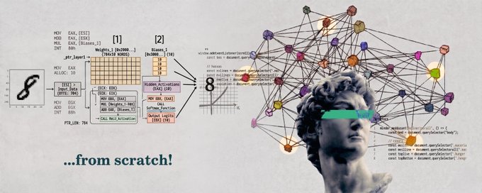
Yeah, you read that right. We're doing this at the lowest level possible. In this article we're going to building a tiny XOR neural network in x86-64 assembly. No libraries. No shortcuts. Just you and the CPU.
Prerequisites: You should know the basics of what a neural network is (layers, weights, biases, activation functions). Some assembly experience helps, but I'll explain things as we go. You'll need NASM and GCC installed on a Linux box.
Table of Contents
The Game Plan
Quick Refresher: What Are We Actually Computing?
Setting Up: Data Section and Memory Layout
Step 1: The Forward Pass
Step 2: The Activation Function (Sigmoid)
Step 3: Computing the Loss
Step 4: Backpropagation
Step 5: Weight Updates
Step 6: The Training Loop
Full Code Listing
Building and Running
1. The Game Plan
We're going to solve the XOR problem. It's the "hello world" of neural networks because a single-layer perceptron can't solve it. You need at least one hidden layer.
Here's the XOR truth table:
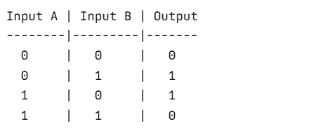
Our network architecture:
That's it. 2 --> 2 --> 1. Tiny, but enough to learn XOR.
2. Quick Refresher: What Are We Actually Computing?
Before we touch assembly, let's be crystal clear about the math. If this is boring to you, skip ahead. If not, read carefully because this is what we're going to translate into instructions.
Forward pass (hidden layer):
Forward pass (output layer):
Loss (mean squared error for one sample):
Backpropagation: We compute how much each weight contributed to the error, then nudge it in the right direction. The chain rule is doing all the heavy lifting here.
For the output layer:
For the hidden layer:
Weight update:
That's the entire algorithm. Now let's make the CPU do it.
3. Setting Up: Data Section and Memory Layout
In assembly, there's no float weights[6]. You manually reserve bytes in the .data or .bss section and keep track of what's where. This is the part where you realize how spoiled high-level languages have made us.
Here's our data section:
Let me explain what's going on here:
- dd means "define double-word", which is 4 bytes, the size of a 32-bit float. Each dd 0.5 reserves 4 bytes and stores the float value 0.5 there.
- resd 1 means "reserve space for 1 double-word", the same 4 bytes but uninitialized. We will write to these during computation.
- Every weight, bias, input, and intermediate value gets its own labeled memory location. In Python you'd just use variables. Here, you're the memory manager.
The training data is laid out flat: 4 samples × 3 floats each = 12 floats = 48 bytes, all sitting in a row. We'll step through them with pointer arithmetic during training.
4. Step 1: The Forward Pass
This is where the actual "thinking" happens. We take inputs, multiply by weights, add biases, and pass through sigmoid. Let's do the hidden layer first.
Stop. Let's talk about the register problem.
This is the #1 thing that bites you in assembly neural nets. In Python, you write h1 = sigmoid(w1*x1 + w2*x2 + b1) and then x1 is still x1. In assembly, calling a function like sigmoid can destroy your register values. The System V AMD64 calling convention says xmm0-xmm7 are caller-saved, meaning any function call can overwrite them.
So we need to save our inputs to memory before calling sigmoid, then reload them. Here's the corrected version:
Let's break down the key instructions you're seeing:
- xmm0, [w1]: Load a 32-bit float from memory address w1 into register xmm0
- mulss xmm2, xmm0: Multiply the float in xmm2 by the float in xmm0, store result in xmm2
- addss xmm2, xmm3: Add xmm3 to xmm2
- movss [z1], xmm2: Store the float in xmm2 to memory address z1
The ss suffix means "scalar single-precision", so we are operating on one 32-bit float at a time. If we wanted to go faster, we would use ps (packed single) to process 4 floats at once with SIMD. But let’s learn to walk before we run.
5. Step 2: The Activation Function (Sigmoid)
The sigmoid function is σ(x) = 1 / (1 + e^(-x)). This is where things get interesting because assembly doesn't have an exp() instruction.
Well, technically x87 FPU has f2xm1 which computes 2^x - 1, and we can use the identity e^x = 2^(x * log2(e)) to build exp() from that. It's gross but it works.
Yeah. That's a lot of code for 1/(1+exp(-x)). Welcome to assembly.
Let me walk through what the x87 FPU stuff is doing, because it probably looks like alien language:
The x87 FPU is a stack-based floating-point unit that's been around since the 8087 coprocessor in 1980. It uses a stack of 8 registers called ST0 through ST7. You push values on, do operations, and pop results off.
- fld dword [rsp]: push a 32-bit float from memory onto the FPU stack
- fldl2e: push the constant log₂(e) onto the stack (the CPU literally has this built in)
- fmulp: multiply ST0 × ST1, pop both, push the result
- frndint: round ST0 to the nearest integer
- f2xm1: compute 2^(ST0) - 1 (only works for ST0 in [-1, 1])
- fscale: compute ST0 × 2^(ST1) (this is how we recombine the integer and fractional parts)
The trick with f2xm1 is that it only works for inputs between -1 and 1. So we split our exponent into integer + fraction parts, compute 2^fraction with f2xm1, then scale by 2^integer with fscale. This is a standard technique.
6. Step 3: Computing the Loss
The loss tells us how wrong we are. We use mean squared error: loss = 0.5 * (target - output)^2. We also need the raw error for backprop.
Yep. One instruction plus the ret. After all that sigmoid pain, this feels nice.
We do not actually need to compute the full loss value for training; we only need the error for backprop. But if you want to track the loss for printing:
7. Step 4: Backpropagation
This is the hardest part conceptually, but in assembly it is really just more multiplies and subtracts. We need to compute the gradients, which tell us how much each weight needs to change.
Remember, the sigmoid derivative has a nice property: σ'(x) = σ(x) * (1 - σ(x)). Since we already have σ(x) stored from the forward pass, we do not need to recompute anything.
Notice the pattern? Each delta computation is the same structure:
This is the chain rule in action. The gradient "flows backward" through each connection, getting multiplied by the local derivative at each step. In Python this is one line with autograd. Here, you see every multiply.
8. Step 5: Weight Updates
Now we nudge every weight in the direction that reduces the error. The update rule is:
This is tedious but straightforward. Every weight update is the same three instructions: load, multiply, add-to-existing-weight. Nine weights and biases = nine little update blocks.
You can see why people invented matrix libraries.
9. Step 6: The Training Loop
Now we wire everything together. For each epoch, we loop through all 4 training samples, run forward pass → compute error → backprop → update weights.
A few things to notice:
Pointer arithmetic: We use r14 as a pointer into the training data and advance it by 12 bytes (3 floats × 4 bytes) after each sample. This is how you "iterate over an array" in assembly.
cvtss2sd: printf expects double (64-bit) arguments for %f, but we've been working with float (32-bit) everywhere. So we have to convert before printing. Classic C ABI headache.
mov rax, 4: The System V AMD64 calling convention requires you to put the number of XMM register arguments in rax before calling variadic functions like printf. Forget this and you'll get garbage output or a segfault.
10. Full Code
Here's the complete program in one block. Save this as nn.asm:
11. Building and Running
Expected output (values will be approximate):
The outputs will not be exactly 0 and 1 because the sigmoid never quite reaches those values, but they should be close. If your outputs are all around 0.5, the network did not converge. Try different initial weights or increase the number of epochs.
Where to Go From Here
- Add ReLU instead of sigmoid. It's way simpler in assembly and trains faster.
- Use SIMD (packed operations) to process multiple neurons at once. Replace mulss with mulps and watch your hidden layer compute in one instruction instead of two.
- Write the weight initialization using a random number generator instead of hard-coded values.
Keep building. Keep learning.
## 相关链接
- [vixhaℓ](https://x.com/TheVixhal)
- [@TheVixhal](https://x.com/TheVixhal)
- [27K](https://x.com/TheVixhal/status/2044818391240995033/analytics)
- [Upgrade to Premium](https://x.com/i/premium_sign_up)
- [12:41 AM · Apr 17, 2026](https://x.com/TheVixhal/status/2044818391240995033)
- [27.4K Views](https://x.com/TheVixhal/status/2044818391240995033/analytics)
- [View quotes](https://x.com/TheVixhal/status/2044818391240995033/quotes)
---
*导出时间: 2026/4/17 15:36:16*