Build Your Own Virtual Machine in Under 200 Lines of C ✍ Scarlett🕐 2026-04-20📦 33.0 KB 🟢 已读 𝕏 文章列表 这是一篇关于如何从零开始构建虚拟机的教程。作者旨在用不到 200 行的 C 语言代码实现一个简易的进程虚拟机。文章基于冯·诺依曼架构和 LC-3 教学架构,详细介绍了虚拟机的内存模型、寄存器设计、指令系统格式以及程序的加载与执行流程,旨在帮助读者深入理解计算机底层的运行原理。 C语言虚拟机计算机原理LC-3底层开发系统架构编程实战LLVM # Build Your Own Virtual Machine in Under 200 Lines of C **作者**: Scarlett **日期**: 2026-04-19T17:22:52.000Z **来源**: [https://x.com/Zyara_1ot/status/2045916052559900725](https://x.com/Zyara_1ot/status/2045916052559900725) ---  You’re not just reading this, you're about to build your own Virtual Machine. No dependencies. No frameworks. No abstractions. Just raw C. By the end, you'll have a VM that can read instructions, manipulate memory, and control its own execution flow. This is not a quick skim. We're going deep, step by step. So make sure you come prepared with: - patience - time - and understanding of c and bit manipulation I'll try to keep everything as simple and intuitive as possible. No sudden jumps, just a smooth, structured build from scratch. ## Contents - Introduction - Architecture Overview - VM Design and Implementation Core Components - Main Memory - Registers - Data Model Instruction System - What is a CPU Instruction? - Instruction Format - Supported Instruction Set - Breakdown instruction System Interaction - TRAP Mechanism - Supported TRAP Functions Putting It All Together - Implementation Walkthrough - Building and Running the Program ## Introduction VIRTUAL MACHINE A virtual machine is a system that emulates a computer architecture or system. There are two main catagories of Virtual machines: - System Virtual Machines : emulate a full computer, allowing entire operating systems to run on them. - Process Virtual Machines : run individual programs in a platform independent way (e.g. Java Virtual Machine). What we will build is a simple process virtual machine. that can execute programs in a platform-independent environment. Inspired by the LC-3 architecture, our VM will interpret and run a subset of LC-3 assembly instructions. > LC-3 (Little Computer 3) is a simple, educational assembly language and architecture. It's way easier than x86 but still has enough features to write decent programs and understand how real systems work. > For simplicity, we're stripping out a lot of advanced stuff interrupts, priority levels, PSR (process status registers) , privilege modes, and stacks. We'll keep only the core hardware and handle input/output through traps. ## Architecture Overview Our LC-3 inspired VM follows the von Neumann model, just like most real computers. It has three main parts: CPU, memory, I/O. - CPU (central processing unit) : This is where all the action happen. It controls and manipulates data. CPU is further divided into 3 parts: ALU (Arithmetic Logic Unit) : represents the circuits that actually carry out the instructions on the data (performing operations like add, not etc). CU (control unit) : coordinates the activities within the CPU. Registers : tiny, super-fast storage where all computations happen (data from a memory location into a register, performing some operations on it, and then storing the result back into memory.) . We don't operate directly on memory because it's slow and the CPU is designed to perform computations using registers. - Main memory : its just a big array of values. It stores both instructions and data in binary form. imagine it as an array of W words , each word is of N bits. Each word contains either 1 instruction or a program data. - I/O : enable the computer to communicate with the outside world. 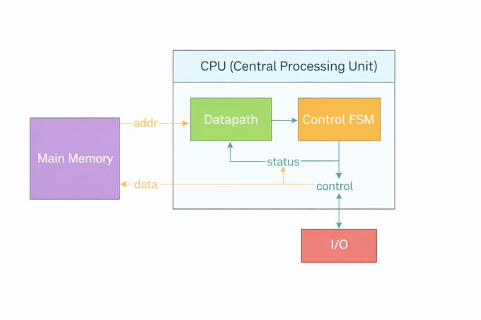 model ## VM Design and Implementation How our VM works : Load the program into main memory point the rpc register (we will discuss it) at the first instruction read the instruction decode execute and move to the next (increment rpc) 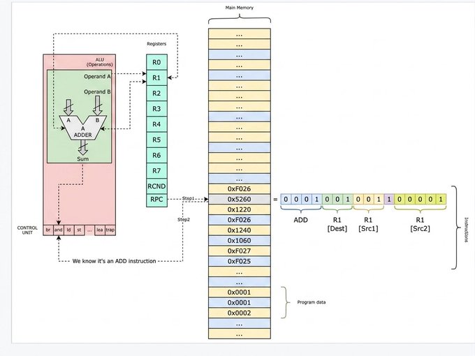 execution - MAIN MEMORY This is the memory space of our VM. consisting of W = uint16_max words each N = 16bits wide. The constant UINT16_MAX represents the maximum value of an unsigned 16-bit integer, which is 65535. By adding 1 to the array size, we create exactly 65,536 addressable slots (ranging from 0x0000 to 0xFFFF). each slot holds 16bits , so total its 128kb. First it might seems like, its quite constrained , cause it can't load programs exceeding 65,536 instructions or data words. But it will make you shock that , even with this much constraints , it provide enough space to store several ASCII games and their associated data entirely in memory. By convention, we begin loading programs at address 0x3000. The memory region below 0x3000 is reserved for potential system components. Let's discuss a little bit of memory layout here: All the 65536 address aren't free for our program. The reserved slots are : 0X0000 - 0X00FF - > Trap vector table (trap routine address) 0X0100 - 0X01FF - > Interrupt vector table 0X0200 - 0X2FFF - > OS / Supervisor space 0X3000 - 0XFDFF - > user program space (our program loads here) 0XFE00 - 0XFFFF - > memory mapped I/O > *****Let me tell you something cool here, what did we discuss earlier? that our main memory is a large array, and here look, we are taking blocks of contiguous memory and reserving them for different purposes, if you translate those hex values to numbers you will see, 0 to 255 - > for trap ,and just next ,, 256 to 511 - > Interrupt vector table,, like that . cool isn't it? To interact with the memory, we will use two helper functions for reading (mr) and writing (mw): - REGISTERS Our VM features a total of 10 registers, each 16 bits wide: - R0 is a general-purpose register. It is also used for reading and writing data to and from stdin and stdout. - R1 through R7 are additional general-purpose registers (most of the computation happens here) . - RPC (Program Counter) is the register that holds the memory address of the next instruction to be executed. - RCND (Condition Flag) is the conditional register. It stores status flags that provide information about the result of the most recent operation performed by the ALU. we can implement the register set as an array and use an enum to define the indices for better readability: AND NOW COMES THE ACTUAL INTERESTING PART ; - INSTRUCTION SYSTEM > What is a CPU instruction? - > Instructions are nothing but the command we give to the VM. same word size as the memory, 16 bits. an instruction is just a number, carefully structured to pack multiple pieces of information into 16 bits In our VM, instructions are 16 bits wide, matching the size of a memory word. Since instructions are stored in memory, this alignment keeps things simple. Here, we represent each instruction using a uint16_t. The VM supports a compact instruction set of 16 operations (effectively 14, since two LC-3 instructions aren’t needed in this implementation). Instruction format : We will use the following format to encode instructions into a uint16_t : The basic pattern: 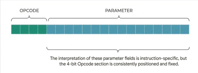 Hmmmmm so many opcode opcode right?? Lets see what is it. OPCODE : means operation code. A number that selects which circuit should run. A machine executes many different kinds of actions: add, and , not, jump, call etc.. . The machine needs a way to answer the first question every time it sees an instruction: what kind of instruction is this?? OPCODE answer this. In every 16 bits , the first 4 bits represent opcode of the instruction. Its like, extract first 4 bits and you know the operation. To extract the OpCode, we use a utility macro that employs a simple bitwise shift: By shifting 12 bits to the right (i >> 12), we isolate the 4 most significant bits. (I hope you are able to understand , already told you to sit with bit manipulation understanding) OpCodes are 4 bits wide, we can encode a maximum of 16 unique instructions (2^4 = 16). **A powerful trick for organizing our VM is to store all possible instructions and their associated C functions in an array. The array index represents the OpCode (0 to 15), and the value is a pointer to the corresponding C function. By defining a function pointer type, we can map each opcode directly to its corresponding instruction handler, avoiding a large and messy switch statement. Each instruction is fetched from memory using the program counter, and then immediately dispatched using: Here, OPC(i) extracts the opcode, which acts as an index into the op_ex table. Each entry in this table points to a function that implements a specific instruction. For example, if the opcode is 0b0001, the VM calls add(i). If it is 0b0010, it calls ld(i). OK OK , I KNOW WHAT YOU AR THINKING, WHAT ARE THERE DIFFERENT INSTRUCTIONS?? Here you go. Supported Instruction Set The following table lists the instructions supported by our VM, based on the LC-3 specification: 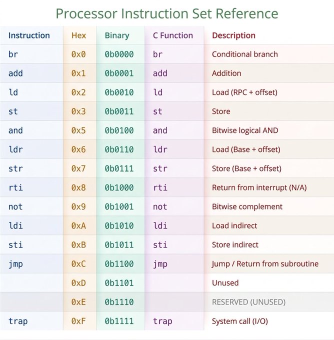 These can be grouped into four categories: - Control Flow: br, jmp, and jsr manage jumping and conditional logic (similar to if or goto). - Memory Loading: ld, ldr, ldi, and lea move data from memory into registers. - Memory Storage: st, str, and sti move data from registers back to memory. - Mathematical Operations: add, and, and not process data within registers. The trap instruction is unique; it handles I/O, allowing the VM to read from stdin and write to stdout. Conditional flags (RCND) : RCND is just a register. like R0-R7, it's a uint16_t slot in your register array. but unlike general purpose registers, it has one specific job , it remembers the "mood" of the last result. it holds one of three values at any time: - FN = 1<<2 = 4 → last result was negative - FZ = 1<<1 = 2 → last result was zero - FP = 1<<0 = 1 → last result was positive exactly one is set at all times. never two, never zero. why do we need it our VM has no comparison instruction. there's no CMP R0, R1 that directly says "is R0 greater than R1?" so how do we do an if statement? how do we do a loop? we do arithmetic, then check RCND. want to check if R0 == 0? just do any operation that puts R0's value into a register. if RCND becomes FZ, it's zero. want to check if a > b? subtract: a - b. if result is positive, FP is set → a was bigger. if negative, FN is set → b was bigger. if zero, FZ → they're equal. then BR (hold up, we will discuss) reads RCND and decides whether to jump. why not just compare directly because at the hardware level, comparison IS subtraction. every CPU works this way , x86 has a (comparison instruction) CMP instruction but under the hood it's just subtraction that discards the result and keeps the flags. LC-3 just makes that explicit instead of hiding it. RCND is the bridge between arithmetic and control flow. without it, you can't do loops, if statements, or any conditional logic. it's small but the entire branching system depends on it. we update these flags with a helper function: We call uf(r) after any instruction that modifies a register and affects condition codes. ## What Each Instruction Actually Does Before start explaining all the instructions, lets discuss a little about instruction format. I told you about its basic pattern, lets do a little deep dive into it. What we had was [opcode] | [parameters] Now here, OPCODE we have seen, 4 bits , represent an instruction. What about the parameters? what do they do? and how? Let's see..... It would be better if we take an example and understand while decoding it . Let's take a real instruction from memory: 0x1283. Right now, it's just a hexadecimal number. Let's transform it into something meaningful. Step 1: Convert to Binary First, we need to see the actual bits: 0x1283 in hexadecimal. Each hex digit = 4 binary bits: 1 - 0001 2 -0010 8 - 1000 3 - 0011 Result: 0001 0010 1000 0011 Step 2: Extract the OpCode Remember, the OPCODE is the first 4 bits (positions 15–12): 0001 0010 1000 0011 These 4 bits = 0001 = 1 (decimal) Looking at our instruction table, OpCode 1 is… ADD! So we know this instruction performs an addition. But ADD between what and what? Here comes the parameters in picture. Step 3: Extract the Parameters The instructions use this format : [OpCode] [DR] [SR1] [Mode] [SR2 or IMM5] where: DR : Destination Register (where result goes) SR: Source Register (operand: a value an instruction operates on) MODE: 0 for register mode, 1 for immediate mode.{ Register mode : operand comes from register, immediate mode: operand is embedded in the instruction itself. But, We call it a MODE when we talk about behavior. We call it FIMM when we talk about bits.} IMM5: An immediate value stored using 5 bits. (why 5?? After opcode, DR, SR, MODE selector, 5 bits left) FIMM: Immediate flag, that tells the cpu wheather the instruction uses an immediate value or not. Actually, FIMM has the 0/1 values. The mode is the behavior those values select. Let's breakdown the 16 bits : - Bits [15:12] = 0001 = OPCODE (4 bits) - Bits [11:9] = 001 = Register 1 (R1) <- destination (DR) (3 bits) - Bits [8:6] = 010 = Register 2 (R2) <- first operand (SR1) (3 bits) - Bit [5] = 0 = Register mode (FIMM = 0) <- mode selector (1 bit) - Bits [4:3] = 00 = padding (ignored in register mode) (2 bit) - Bits [2:0] = 011 = Register 3 (R3) ← second operand (SR2) (3 bit) > **** Here look, The last 5 bits don’t change, but how we read them does. If we're in register mode (FIMM = 0), we ignore the first 2 bits and use the last 3 bits as a register (SR2). If we're in immediate mode (FIMM = 1), we take all 5 bits together as a number (IMM5). So the bits stay the same, the meaning changes based on FIMM. > That's what makes this design efficient: one instruction format, two behaviors, no extra bits wasted. 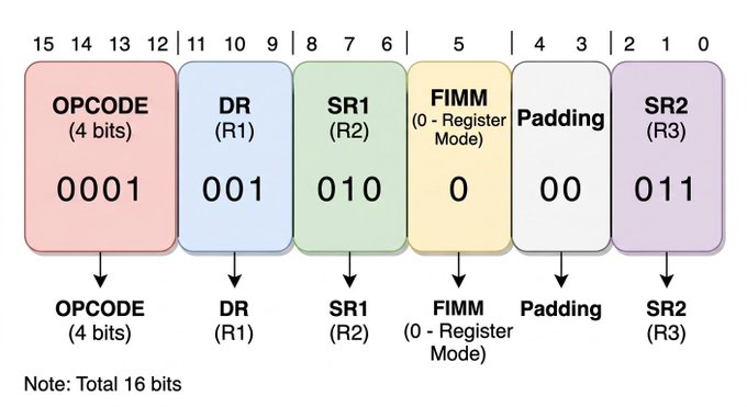 Step 4: The Complete Instruction Putting it all together: 0x1283 = ADD R1, R2, R3 In plain English: "Take the value in R2, add it to the value in R3, and store the result in R1." Let's breakdown all the instructions now one by one : - ADD : Adding two values The ability to add numbers is fundamental to any CPU. In our VM, we define two variations of the add instruction. While they share the same OpCode, their encoding differs based on the value of bit[5], which determines how the second operand is interpreted. The first variation (register mode) adds the values of two source registers, SR1 and SR2, and stores the result in the destination register, DR1: 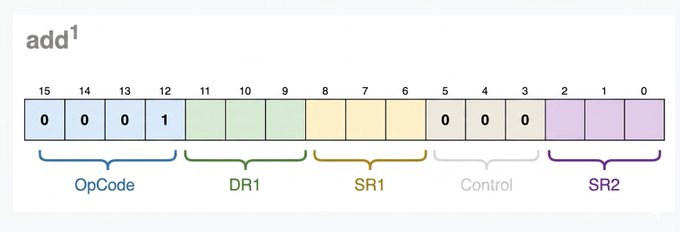 The second variation (immediate mode) adds a “constant” 5-bit value (IMM5) to SR1 and stores the result in DR1: 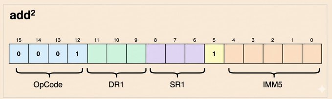 **Before we use immediate values, we need a way to correctly interpret them as signed numbers. We implement a sext (sign extend) function to handle this: Sign Extension (SEXT) : We use sign extension to turn a small immediate into a proper 16-bit signed value. We implement a sext (sign extend) function to handle this: SEXTIMM(i) operates like this for negative numbers: Let's break this down: DR(i) extracts bits [11:9] - the destination register, where the result will be stored. SR1(i) extracts bits [8:6] - the first source register. FIMM(i) checks bit [5] - if it's 1, we're in immediate mode. if it's 0, register mode. in immediate mode - SEXTMM(i) extracts the 5-bit immediate value and sign-extends it to 16 bits so it can be treated as a proper signed number. in register mode - SR2(i) extracts bits [2:0] , the second source register. finally, uf(DR(i)) updates the condition flags based on whatever value just landed in DR. so the entire instruction - decode operands, pick mode, compute result, update flags - happens in one line. that's the payoff of defining clean macros upfront. 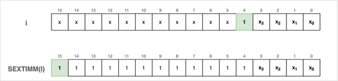 To verify this logic , we can take an example: To see if its immediate mode or register mode , we extract the 5th bit using bit-mask. 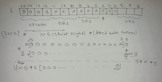 We use simple bitwise macros to extract different fields from the 16-bit instruction. Each macro shifts the relevant bits into position and masks out everything else. The idea is straightforward: we first shift right to bring the desired bits to the least significant position, and then mask using a bit pattern to keep only those bits. By combining all these , the add function checks the FIMM flag to decide whether to add a second register or a sign-extended immediate value. Finally, it updates the condition flags (uf) based on the result. - AND : This instruction is functionally very similar to add, and it likewise comes in two formats. The first format (register mode) applies a bitwise AND (&) to the values of two registers, SR1 and SR2, storing the result in DR1 : [OPCODE] [DR1] [SR1] [000] [SR2] The second format (immediate mode) applies a bitwise AND between SR1 and a sign-extended IMM5 value, storing the result in DR1: [OPCODE] [DR1] [SR1] [1] [IMM5] same as before, we check bit[5] to determine which format to decode. Implementation is nearlyy identical too, we just simply swap (+) for the (&). - ld - LOAD RPC + offset Here, we use the RPC (Program Counter) as a reference point to access memory. Instead of storing a full memory address inside the instruction, we compute the target address by adding an offset to the current RPC. An offset simply tells us how far the desired location is from the current one, positive values move forward in memory, while negative values move backward. why this design ? - > because storing full addresses would require more bits and make instructions larger. By using a small signed 9-bit offset, we keep instructions compact while still being able to access nearby memory efficiently. The tradeoff is reach a 9-bit signed offset can only access addresses within -256 to +255 words of the current RPC. For data that lives far away in memory, we have ldi , but we'll get to that. For example, if the RPC currently points to the memory address 0x3002 and our offset is set to 100, the VM will read the data from location 0x3002 + 100 = 0x3066 and load it into the specified destination register. ld : [OPCODE] [DR1] [OFFSET9] The offset in the LD instruction is 9 bits wide, which means it can represent 29=5122^9 = 51229=512 different values. Since the offset is signed (two’s complement), its actual range is from −256 to +255.his means that depending on where your program is located in memory, large sections of the address space may remain inaccessible to the ld instruction. To overcome this addressability limitation, we need to introduce another instruction called ldi. - LDi : Load Indirect we use ldi , when data is far away, or not reachable using ld. The idea is something like , Instead of loading data directly, LDI first fetches an address from memory, and then loads the value from that address. Let’s take an example: suppose the RPC points to 0x3002. Just like with the ld instruction, we use a 9-bit signed offset to calculate a target address. If the offset = 100, the VM first looks at the memory address 0x3002 + 100 = 0x3066. However, instead of loading the value 0x3066 into our destination register, the VM treats the content of 0x3066 as another address. If 0x3066 contains the value 0x3204, the VM performs a second read at 0x3204 and brings that data into the DR. By using this "pointer" logic, ldi allows your program to access any location in the 16-bit address space, regardless of where the current RPC is. **It doesnt mean ldi is always better than ld, it has its own tradeoffs, ld is fast, ldi performs 2 operations , its slow. LDi : [OPCODE] [DR1] [OFFSET9] - LDr (Load Base + offset) : unlike ld which calculates the address relative to the RPC, ldr allows us to specify a custom base address, specifically, a memory address already stored in one of our general-purpose registers. ldr : [OPCODE] [DR1] [BASER] [OFFSET6] To extract the BASER (the register holding the base address) from the instruction, we can reuse the SR1(i) macro we defined earlier for ld, as the bits occupy the exact same positions. To extract the OFFSET6 ( a 6-bit signed offset), we use a new macro that isolates the last 6 bits and applies sign extension: implementation is nearly identical to ld, just change in reference - lea : Load Effective Address This instruction is used to load raw memory address into register. key difference between ld, ldr, ldi , and lea is , those fetch the content stored t an address, but LEA does not load data from memory, it loads an address itself into a register. the instruction operates as a simple calculation relative to PC (program counter). address = RPC + offset DR = address lea : [OPCODE] [DR1] [OFFSET9] - NOT - Bitwise NOT operation : This instruction performs not operation on on the value stored in the source register SR1 and saves the result in the DR. not : [OPCODE] [DR1] [SR1] [1 1 1 1 1 1] In this operation, every 0 in the source bitmask is flipped to a 1, and every 1 is flipped to a 0. Since this operation modifies the contents of a register, we must also update the condition flags. - ST - Store Operation This instruction stores the value from a register into memory. st : [OPCODE] [SR] [offset9] This instruction takes the value stored in the source register and writes it to a memory location. The target address is not stored directly; instead, it is computed by adding a signed offset to the current RPC (Program Counter). In other words, we use RPC as a reference and determine where to store the value based on how far (offset) the target location is from the current instruction. Since this operation only writes to memory and does not modify any register values, the condition flags are not updated. - STI - Store Indirect This instruction is similar to ST, but instead of storing the value directly at the computed address, it uses that location as a pointer. sti : [OPCODE] [SR] [PCoffset9] Like ST, we use RPC as a reference and compute an address using an offset. However, in this case, we do not store the value at that address directly. Instead, we first read a new address from that location, and then store the value at this final address. So unlike ST (one step), STI performs an extra level of indirection. Since this operation only writes to memory and does not modify any register values, the condition flags are not updated. STR - Store (Base + Offset) This instruction is similar to ST, but instead of using RPC as the reference, it uses a base register. str : [OPCODE] [SR] [BaseR] [offset6] Like ST, we store a value from a register into memory. However, instead of computing the address using RPC, we use a base register (SR1) and add a small offset to it. So the address is determined relative to a register rather than the current instruction location. again same, only write so, doesnt modify any register value, conditional flags. - jmp - JUMP normally, the RPC automatically increments after each instruction is executed, leading to a linear flow of execution. But what if the target is not relative to current position, what if we need to jump to a new memory address. For all these situation, we will use jmp. The target address is not relative to the current position; instead, it is the exact value currently stored in a Base Register (BASER). jmp : [OPCODE] [0 0 0] [BASER] [0 0 0 0 0 0] For example, if RPC is at 0x3005 and the base register contains 0x3010, executing JMP will immediately set RPC to 0x3010. The very next instruction executed will be from that address. In high-level terms, this behaves like a low-level goto, allowing control flow changes such as loops, branching, or jumping to different parts of the program. Since this instruction only updates the RPC and does not modify any data registers, the condition flags are not updated. - jsr - jump to subroutines The jsr (Jump to Subroutine) instruction is what enables function-like behavior in our virtual machine. A subroutine is simply a block of instructions designed to perform a specific task, usually taking input from registers and producing a result in a register. jsr is unique because it doesn’t just jump; it “remembers” where it came from so the program can eventually return to the next instruction after the function call. This instruction supports two formats: - JSR (PC-relative): The target address is computed by adding an offset to the current RPC. This is useful for jumping to nearby code. bit[11]=1 - JSRR (register-based): The target address is taken directly from a base register, allowing jumps to arbitrary locations stored in registers. bit[11] = 0 jsr : [OPCODE] [1] [OFFSET11] jsrr : [OPCODE] [0][00] [BASER] [000000] We use a macro FL(i) to check the state of bit 11 and POFF11(i) to extract and sign-extend the larger 11-bit offset. - BR - Branch This instruction changes the flow of execution based on condition flags. br : [OPCODE] [cond flags] [PCoffset9] Unlike JMP, which always jumps, BR performs a conditional jump. It checks the condition flags stored in RCND (Negative, Zero, Positive) and decides whether to branch. We again use RPC as a reference and compute the target address using an offset. However, this jump only happens if the specified condition matches the current flags. For example, if the result of a previous operation was negative, the N flag is set. A BRn instruction will then cause a jump, while others will not. If the condition is satisfied: RPC = RPC + offset Otherwise, execution continues normally with the next instruction. ## System Interaction - TRAP Mechanism The trap instruction is one of the most important parts of our VM because it acts as the bridge between our virtual machine and the outside world. Without it, our programs would have no way to interact with I/O devices like the keyboard or the console. In a real LC-3 system, the TRAPVECT (lower 8 bits of the instruction) is used as an index into a table stored in memory, where each entry points to a service routine written in assembly. To keep things simple, we take a shortcut: instead of storing these routines in memory, we directly map trap vectors to C functions using an array of function pointers. This allows us to use the C standard library for tasks like input and output, making our implementation much cleaner. TRAP Dispatcher : We handle traps in a way similar to instruction execution , using a lookup table. Here: - TRP(i) extracts the trap vector - we subtract 0x20 because LC-3 traps start from 0x20 - the result directly indexes into our function table SUPPORTED TRAP FUNCTIONS : Our VM supports 8 distinct trap routines, Let's implement them now: IMPLEMENTATION - tgetc & tout : These handle single-character I/O. Note that for tout, we cast the register value to a char. - tputs : This treats memory as a C-style string. It starts from the address stored in R0 and keeps printing characters until it encounters a null terminator (0x0000). - tin : Short form of “Trap IN”. This reads a character from input and immediately echoes it back to the console. - thalt : Stops the execution of the VM by breaking the main loop. - tinu16 & toutu16 : These are custom helpers for handling 16-bit integers directly using standard I/O. > tputsp : we leave this unimplemented , if you want a challenge, this is yours to fill in. ## Putting it All Together Implementation Walkthrough We have already covered almost the whole part, so congratulations if you are with us till now. To finalize the project, we only need to implement two remaining components: the main execution loop and a mechanism to load binary programs into memory. The instruction cycle (main loop) At the core of our VM lies the fetch decode execute cycle, which drives the entire execution process. Once a program is loaded into memory, the VM repeatedly performs these three steps until a HALT instruction stops execution. We begin by initializing the RPC to the starting address of the program. By convention, programs are loaded at 0x3000, so execution begins from there (with an optional offset). Inside the loop: - Fetch: We read the instruction from memory at the address pointed to by RPC. Immediately after fetching, RPC is incremented so it points to the next instruction. - Decode & Execute: The opcode is extracted from the instruction, and using it, we directly call the corresponding handler function from our function pointer table (op_ex). This loop continues as long as the VM is running. When a HALT trap is executed, the running flag is set to false, and the loop terminates. Loading the Program Image To execute a program, we first need to bring it from disk into our VM’s memory. This is handled by the ld_img function, which reads a binary file (.obj) and loads its contents directly into the mem array starting at our program entry point. We open the file in binary mode, position a pointer at 0x3000 (plus any offset), and then read the contents sequentially into memory. This effectively simulates loading a program into RAM before execution. What it takes : - fname - path to the .obj file - offset - optional shift from the default load address (0x3000) The Entry Point Finally, everything comes together in the main function. This is where we connect loading and execution into a complete flow. The program takes the path to a compiled .obj file as a command-line argument. It first loads this binary into the VM’s memory, and then starts the execution loop. If no file is provided, we print a usage message and exit to avoid undefined behavior. What happens step-by-step : Take program file from command line Load it into memory at 0x3000 Initialize RPC Begin execution loop Running program our first program our first program will be something like : a small program that reads two numbers from the keyboard and prints their sum. At the machine level, the program is simply a sequence of 16-bit values: Yeah, this raw representation isn’t very readable, it’s just a list of hexadecimal numbers. But each value encodes a full instruction, and once we decode it, the structure becomes clear. But remember how we decode the hex value, just like that you can decode these values manually too , once maybe for fun. here's one from my side: 0x1240 - 0001 001 001 0 00000 ADD R1 R1 R0 Here: - FIMM = 0 - register mode - last 3 bits - R0 Meaning: R1 = R1 + R0 Running our first program : Bad news: we don't have a compiler or assembler for our instruction set yet. That means we can't write programs in a high-level syntax and compile them automatically, we have to work directly with raw machine code. The good news is that we don't actually need a full toolchain. Since our VM expects a binary file containing 16-bit instructions, we can generate that file ourselves using a small C program. The idea is simple: store our instructions in a uint16_t array and write them directly to a file using fwrite(). This file then becomes the program image that our VM can load and execute. If you compile and run this packer, it will generate a file named sum.obj. You can then use your VM to load and execute it. > And that's it. You built a working virtual machine. From scratch. In under 200 lines of C. > Where to go from here , write more programs for your VM, try implementing a loop or a function call in raw machine code. Implement tputsp, we left it empty on purpose. Try adding your own instruction using the two empty opcode slots sitting there doing nothing (RTI, RES). Or go wild and build a simple assembler so you never have to hand-encode hex again. GOOD LUCK! [Repo link in replies] ## 相关链接 - [Scarlett](https://x.com/Zyara_1ot) - [@Zyara_1ot](https://x.com/Zyara_1ot) - [6.1K](https://x.com/Zyara_1ot/status/2045916052559900725/analytics) - [jmp](https://www.andreinc.net/2021/12/01/writing-a-simple-vm-in-less-than-125-lines-of-c/#jmp---jump) - [ldr](https://www.andreinc.net/2021/12/01/writing-a-simple-vm-in-less-than-125-lines-of-c/#ldr---load-baseoffset) - [ldi](https://www.andreinc.net/2021/12/01/writing-a-simple-vm-in-less-than-125-lines-of-c/#ldi---load-indirect) - [lea](https://www.andreinc.net/2021/12/01/writing-a-simple-vm-in-less-than-125-lines-of-c/#lea---load-effective-address) - [str](https://www.andreinc.net/2021/12/01/writing-a-simple-vm-in-less-than-125-lines-of-c/#str---store-base--offset) - [sti](https://www.andreinc.net/2021/12/01/writing-a-simple-vm-in-less-than-125-lines-of-c/#sti---store-indirect) - [add](https://www.andreinc.net/2021/12/01/writing-a-simple-vm-in-less-than-125-lines-of-c/#add---adding-two-values) - [and](https://www.andreinc.net/2021/12/01/writing-a-simple-vm-in-less-than-125-lines-of-c/#and---bitwise-logical-and) - [not](https://www.andreinc.net/2021/12/01/writing-a-simple-vm-in-less-than-125-lines-of-c/#not---bitwise-complement) - [Upgrade to Premium](https://x.com/i/premium_sign_up) - [1:22 AM · Apr 20, 2026](https://x.com/Zyara_1ot/status/2045916052559900725) - [6,146 Views](https://x.com/Zyara_1ot/status/2045916052559900725/analytics) --- *导出时间: 2026/4/20 17:44:02* --- ## 中文翻译 # 用不到200行C代码构建你自己的虚拟机 **作者**: Scarlett **日期**: 2026-04-19T17:22:52.000Z **来源**: [https://x.com/Zyara_1ot/status/2045916052559900725](https://x.com/Zyara_1ot/status/2045916052559900725) ---  你不仅仅是在阅读这篇文章,你即将构建属于你自己的虚拟机。没有依赖项。没有框架。没有抽象层。只有纯粹的 C 语言。完成之后,你将拥有一个能够读取指令、操作内存并控制自身执行流程的虚拟机。这不是一篇快速浏览的文章。我们要深入探讨,一步一步来。所以请确保你做好了准备: - 耐心 - 时间 - 以及对 C 语言和位操作的理解 我会尽量让一切变得简单直观。没有突如其来的跳跃,只有从零开始、流畅且结构化的构建过程。 ## 目录 - 简介 - 架构概览 - 虚拟机设计与实现 核心组件 - 主内存 - 寄存器 - 数据模型 指令系统 - 什么是 CPU 指令? - 指令格式 - 支持的指令集 - 指令详解 系统交互 - TRAP 机制 - 支持的 TRAP 函数 整合所有内容 - 实现演练 - 构建和运行程序 ## 简介 虚拟机 虚拟机是一种模拟计算机架构或系统的系统。 虚拟机主要有两大类: - 系统虚拟机:模拟完整的计算机,允许在其上运行整个操作系统。 - 进程虚拟机:以平台无关的方式运行单个程序(例如 Java 虚拟机)。 我们要构建的是一个简单的进程虚拟机,它可以在独立于平台的环境中执行程序。受 LC-3 架构的启发,我们的虚拟机将解释并运行 LC-3 汇编指令的一个子集。 > LC-3 (Little Computer 3) 是一种简单的、用于教学的汇编语言和架构。它比 x86 容易得多,但仍具备足够的功能来编写像样的程序并理解真实系统是如何工作的。 > 为了简单起见,我们去掉了许多高级内容:中断、优先级、PSR(程序状态寄存器)、特权模式和栈。我们只保留核心硬件,并通过陷阱来处理输入/输出。 ## 架构概览 我们受 LC-3 启发的虚拟机遵循冯·诺依曼模型,就像大多数真实计算机一样。它有三个主要部分:CPU、内存、I/O。 - CPU(中央处理单元):这是所有操作发生的地方。它控制并操作数据。CPU 进一步分为 3 个部分: ALU(算术逻辑单元):代表实际执行指令的电路(对数据执行加、非等操作)。 CU(控制单元):协调 CPU 内部的活动。 寄存器:微小、超快的存储器,所有的计算都在这里发生(将数据从内存位置读入寄存器,对其进行某些操作,然后将结果存回内存)。我们不直接在内存上操作,因为它很慢,而且 CPU 被设计为使用寄存器进行计算。 - 主内存:它只是一个巨大的数值数组。它以二进制形式存储指令和数据。可以把它想象成一个有 W 个字的数组,每个字 N 位。每个字包含 1 条指令或一个程序数据。 - I/O:使计算机能够与外部世界通信。  模型 ## 虚拟机设计与实现 我们的虚拟机是如何工作的: 将程序加载到主内存 将 rpc 寄存器(我们稍后会讨论它)指向第一条指令 读取指令 解码 执行并移动到下一条(增加 rpc)  执行 - 主内存 这是我们虚拟机的内存空间。由 W = uint16_max 个字组成,每个字宽 N = 16 位。 常量 UINT16_MAX 表示无符号 16 位整数的最大值,即 65535。通过将数组大小加 1,我们创建了正好 65,536 个可寻址槽(范围从 0x0000 到 0xFFFF)。每个槽容纳 16 位,所以总共是 128kb。 起初这似乎非常受限,因为它无法加载超过 65,536 条指令或数据字的程序。但令人惊讶的是,即使有这么多限制,它也提供了足够的空间来将多个 ASCII 游戏及其相关数据完全存储在内存中。 按照惯例,我们从地址 0x3000 开始加载程序。0x3000 以下的内存区域保留给潜在的系统组件。 让我们在这里稍微讨论一下内存布局: 所有 65536 个地址并不是都对我们的程序开放。保留的槽有: 0X0000 - 0X00FF - > 陷阱向量表(trap 例程地址) 0X0100 - 0X01FF - > 中断向量表 0X0200 - 0X2FFF - > 操作系统 / 管理员空间 0X3000 - 0XFDFF - > 用户程序空间(我们的程序加载在这里) 0XFE00 - 0XFFFF - > 内存映射 I/O > *****在这里告诉你一件很酷的事情,我们之前讨论了什么?我们的主内存是一个大数组,这里看,我们正在获取连续的内存块并将它们用于不同的目的,如果你将这些十六进制值转换为数字,你会看到,0 到 255 - > 用于陷阱,就在接下来,,256 到 511 - > 中断向量表,等等。很酷,不是吗? 为了与内存交互,我们将使用两个辅助函数进行读取 和写入: - 寄存器 我们的虚拟机总共有 10 个寄存器,每个都是 16 位宽: - R0 是通用寄存器。它也用于向 stdin 和 stdout 读写数据。 - R1 到 R7 是额外的通用寄存器(大部分计算都在这里发生)。 - RPC(程序计数器)是保存要执行的下一条指令的内存地址的寄存器。 - RCND(条件标志)是条件寄存器。它存储状态标志,提供有关 ALU 执行的最近操作结果的信息。 我们可以将寄存器集实现为一个数组,并使用枚举来定义索引以提高可读性: 现在到了真正有趣的部分; - 指令系统 > 什么是 CPU 指令?- > 指令不过是我们给虚拟机发出的命令。与内存具有相同的字大小,16 位。指令只是一个数字,经过精心结构化以将多条信息打包到 16 位中 在我们的虚拟机中,指令是 16 位宽,与内存字的大小相匹配。由于指令存储在内存中,这种对齐使事情变得简单。这里,我们使用 uint16_t 来表示每条指令。 虚拟机支持一个包含 16 个操作的紧凑指令集(实际上有 14 个,因为在这个实现中不需要两个 LC-3 指令)。 指令格式:我们将使用以下格式将指令编码为 uint16_t: 基本模式:  嗯哼,这么多操作码对吧??让我们看看它是什么。 OPCODE:意思是操作码。一个数字,用于选择应该运行哪个电路。机器执行许多不同类型的操作:加、与、非、跳转、调用等……机器需要一种方法来在每次看到指令时回答第一个问题:这是什么类型的指令??OPCODE 回答了这个问题。在每 16 位中,前 4 位代表指令的操作码。就像,提取前 4 位你就知道了操作。 为了提取 OpCode,我们使用了一个利用简单位移的实用宏: 通过向右移动 12 位 (i >> 12),我们将 4 个最高有效位隔离出来。 (我希望你能理解,已经告诉过你要带着位操作的理解来坐) 操作码是 4 位宽,我们可以编码最多 16 条唯一的指令 (2^4 = 16)。 **组织我们虚拟机的一个强大技巧是将所有可能的指令及其关联的 C 函数存储在一个数组中。数组索引代表操作码(0 到 15),值是指向相应 C 函数的指针。 通过定义一个函数指针类型,我们可以将每个操作码直接映射到其相应的指令处理程序,从而避免使用庞大且混乱的 switch 语句。 每条指令都使用程序计数器从内存中获取,然后立即使用以下方式进行分派: 这里,OPC(i) 提取操作码,它充当 op_ex 表的索引。该表中的每个条目都指向一个实现特定指令的函数。 例如,如果操作码是 0b0001,虚拟机调用 add(i)。如果是 0b0010,它调用 ld(i)。 好了好了,我知道你在想什么,这些不同的指令是什么??给你。 支持的指令集 下表列出了我们的虚拟机支持的指令,基于 LC-3 规范:  这些可以分为四类: - 控制流:br、jmp 和 jsr 管理跳转和条件逻辑(类似于 if 或 goto)。 - 内存加载:ld、ldr、ldi 和 lea 将数据从内存移动到寄存器。 - 内存存储:st、str 和 sti 将数据从寄存器移回内存。 - 数学运算:add、and 和 not 处理寄存器内的数据。 trap 指令是独特的;它处理 I/O,允许虚拟机从 stdin 读取并写入 stdout。 条件标志 (RCND): RCND 只是一个寄存器。像 R0-R7 一样,它是寄存器数组中的一个 uint16_t 槽。但与通用寄存器不同,它有一个特定的工作,它记住最后一个结果的“情绪”。 它在任何时候都持有以下三个值之一: - FN = 1<<2 = 4 → 上一个结果为负 - FZ = 1<<1 = 2 → 上一个结果为零 - FP = 1<<0 = 1 → 上一个结果为正 始终只设置一个。永远不是两个,永远不是零。 为什么我们需要它 我们的虚拟机没有比较指令。没有直接说“R0 大于 R1 吗?”的 CMP R0, R1 指令。 那么我们如何做 if 语句?我们如何做循环? 我们做算术运算,然后检查 RCND。 想检查 R0 == 0 吗?只需执行任何将 R0 的值放入寄存器的操作。如果 RCND 变为 FZ,它就是零。 想检查 a > b 吗?减去:a - b。如果结果为正,则设置 FP → a 更大。如果为负,则设置 FN → b 更大。如果为零,则 FZ → 它们相等。 然后 BR(等一下,我们会讨论)读取 RCND 并决定是否跳转。 为什么不直接比较 因为在硬件级别,比较就是减法。每个 CPU 都是这样工作的,x86 有一个(比较指令)CMP 指令,但在幕后它只是丢弃结果并保留标志的减法。LC-3 只是明确指出了这一点,而不是隐藏它。 RCND 是算术和控制流之间的桥梁。没有它,你就无法做循环、if 语句或任何条件逻辑。它很小,但整个分支系统都依赖于它。 我们用一个辅助函数来更新这些标志: 在任何修改寄存器并影响条件码的指令之后,我们调用 uf(r)。 ## 每条指令实际上是做什么的 在开始解释所有指令之前,让我们先讨论一下指令格式。我告诉过你它的基本模式,让我们稍微深入一点。我们之前有的是 [opcode] | [parameters] 现在,这里,OPCODE 我们已经看过了,4 位,代表一条指令。参数呢?它们做什么?怎么做?让我们看看..... 最好举一个例子并在解码时理解它。 让我们从内存中获取一条真实的指令:0x1283。目前,它只是一个十六进制数。让我们把它转换成有意义的东西。 步骤 1:转换为二进制 首先,我们需要看到实际的位: 十六进制的 0x1283。 每个十六进制数字 = 4 个二进制位: 1 - 0001 2 -0010 8 - 1000 3 - 0011 结果:0001 0010 1000 0011 步骤 2:提取 OpCode 请记住,OPCODE 是前 4 位(位置 15–12):0001 0010 1000 0011 这 4 位 = 0001 = 1(十进制) 查看我们的指令表,操作码 1 是……ADD!所以我们知道这条指令执行加法。 但是是什么和什么之间的 ADD? 这里参数就出现了。 步骤 3:提取参数 指令使用这种格式: [OpCode] [DR] [SR1] [Mode] [SR2 or IMM5] 其中: DR:目标寄存器(结果去的地方) SR:源寄存器(操作数:指令操作的值) MODE:0 表示寄存器模式,1 表示立即数模式。{ 寄存器模式:操作数来自寄存器,立即数模式:操作数嵌入在指令本身中。但是,当我们谈论行为时,我们称之为 MODE。 当我们谈论位时,我们称之为 FIMM。} IMM5:使用 5 位存储的立即数值。(为什么是 5 位??在操作码、DR、SR、MODE 选择器之后,剩下 5 位) FIMM:立即数标志,告诉 CPU 指令是使用立即数值还是不使用。实际上,FIMM 具有 0/1 值。 模式是这些值选择的行为。 让我们分解这 16 位: - 位 [15:12] = 0001 = OPCODE (4 位) - 位 [11:9] = 001 = 寄存器 1 (R1) <- 目标 (DR) (3 位) - 位 [8:6] = 010 = 寄存器 2 (R2) <- 第一个操作数 (SR1) (3 位) - 位 [5] = 0 = 寄存器模式 (FIMM = 0) <- 模式选择器 (1 位) - 位 [4:3] = 00 = 填充(在寄存器模式下忽略)(2 位) - 位 [2:0] = 011 = 寄存器 3 (R3) ← 第二个操作数 (SR2) (3 位) > **** 这里看,最后 5 位不会改变,但我们读取它们的方式会改变。 如果我们在寄存器模式 (FIMM = 0),我们忽略前 2 位,使用最后 3 位作为寄存器 (SR2)。如果我们处于立即数模式 (FIMM = 1),我们将所有 5 位一起作为一个数字 (IMM5)。所以位保持不变,其含义根据 FIMM 变化。 > 这就是使这个设计高效的原因:一种指令格式,两种行为,没有浪费额外的位。  步骤 4:完整的指令 把它们放在一起: 0x1283 = ADD R1, R2, R3 用通俗的英语说:“取 R2 中的值,将其与 R3 中的值相加,并将结果存储在 R1 中。” 现在让我们一个一个地分解所有指令: - ADD:加两个值 加数的能力对任何 CPU 都是至关重要的。在我们的虚拟机中,我们定义了两种加法指令变体。虽然它们共享相同的操作码,但它们的编码根据位 [5] 的值而不同,该值决定如何解释第二个操作数。 第一种变体(寄存器模式)将两个源寄存器 SR1 和 SR2 的值相加,并将结果存储在目标寄存器 DR1 中:  第二种变体(立即数模式)将“常量”5 位值 (IMM5) 加到 SR1 并将结果存储在 DR1 中:  **在我们使用立即数值之前,我们需要一种方法将它们正确解释为有符号数。 我们实现了一个 sext(符号扩展)函数来处理这个问题: 符号扩展 (SEXT):我们使用符号扩展将一个小的立即数变成一个正确的 16 位有符号值。 我们实现了一个 sext(符号扩展)函数来处理这个问题: SEXTIMM(i) 对负数的操作如下: 让我们分解一下: DR(i) 提取位 [11:9] - 目标寄存器,结果将存储在那里。 SR1(i) 提取位 [8:6] - 第一个源寄存器。 FIMM(i) 检查位 [5] - 如果是 1,我们处于立即数模式。如果是 0,则是寄存器模式。 在立即数模式下 - SEXTMM(i) 提取 5 位立即数值并将其符号扩展为 16 位,以便将其视为正确的有符号数。 在寄存器模式下 - SR2(i) 提取位 [2:0],第二个源寄存器。 最后,uf(DR(i)) 根据刚刚落入 DR 的值更新条件标志。 所以整个指令 - 解码操作数、选择模式、计算结果、更新标志 - 都在一行中发生。这就是预先定义干净的宏的回报。  为了验证这个逻辑,我们可以举一个例子: 要看它是立即数模式还是寄存器模式,我们使用位掩码提取第 5 位。  我们使用简单的位宏从 16 位指令中提取不同的字段。每个宏将相关位移入位置并屏蔽掉其他所有内容。 这个想法很简单: 我们首先右移,将所需的位带到最低有效位置,然后使用位模式进行屏蔽,只保留那些位。 通过结合所有这些,add 函数检查 FIMM 标志以决定是添加第二个寄存器还是符号扩展的立即数值。最后,它根据结果更新条件标志 (uf)。 - AND: 这条指令在功能上与 add 非常相似,它也有两种格式。 第一种格式(寄存器模式)对两个寄存器 SR1 和 SR2 的值按位与 (&),并将结果存储在 DR1 中: [OPCODE] [DR1] [SR1] [000] [SR2] 第二种格式(立即数模式)对 SR1 和符号扩展的 IMM5 值按位与,并将结果存储在 DR1 中: [OPCODE] [DR1] [SR1] [1] [IMM5] 和以前一样,我们检查位 [5] 来确定要解码哪种格式。实现也几乎完全相同,我们只是简单地将 (+) 换成了 (&)。 - ld - 加载 RPC + 偏移量 在这里,我们使用 RPC(程序计数器)作为访问内存的参考点。我们没有在指令中存储完整的内存地址,而是通过将偏移量加到当前的 RPC 来计算目标地址。偏移量只是告诉我们所需位置距离当前位置有多远,正值在内存中向前移动,而负值向后移动。 为什么这种设计?- > 因为存储完整地址需要更多的位并使指令变大。通过使用小的有符号 9 位偏移量,我们保持指令紧凑,同时仍然能够高效地访问附近的内存。代价是范围 - 9 位有符号偏移量只能访问当前 RPC 的 -256 到 +255 个字范围内的地址。对于远离内存的数据,我们有 ldi,我们会谈到这一点。 例如,如果 RPC 当前指向内存地址 0x3002 并且我们的偏移量设置为 100,虚拟机将从位置 0x3002 + 100 = 0x3066 读取数据并将其加载到指定的目标寄存器中。 ld:[OPCODE] [DR1] [OFFSET9] LD 指令中的偏移量是 9 位宽,这意味着它可以表示 29=5122^9 = 51229=512 个不同的值。由于偏移量是有符号的(二进制补码),其实际范围是从 −256 到 +255。这意味着根据你的程序在内存中的位置,地址空间的很大部分可能无法被 ld 指令访问。 为了克服这种可寻址性限制,我们需要引入另一条称为 ldi 的指令。 - LDi:间接加载 当数据很远或无法使用 ld 到达时,我们使用 ldi。这个想法有点像,与其直接加载数据,LDI 首先从内存中获取一个地址,然后从该地址加载值。 让我们举个例子:假设 RPC 指向 0x3002。就像 ld 指令一样,我们使用 9 位有符号偏移量来计算目标地址。如果 offset = 100,虚拟机首先查看内存地址 0x3002 + 100 = 0x3066。 然而,虚拟机不是将值 0x3066 加载到我们的目标寄存器中,而是将 0x3066 的内容视为另一个地址。如果 0x3066 包含值 0x3204,虚拟机将在 0x3204 执行第二次读取并将该数据带入 DR。 通过使用这种“指针”逻辑,ldi 允许你的程序访问 16 位地址空间中的任何位置,无论当前的 RPC 在哪里。 **这并不意味着 ldi 总是比 ld 好,它有自己的权衡,ld 很快,ldi 执行 2 个操作,它很慢。 LDi:[OPCODE] [DR1] [OFFSET9] - LDr(加载基址 + 偏移量): 不像 ld 计算相对于 RPC 的地址,ldr 允许我们指定一个自定义基址,具体来说,是已经存储在我们的一个通用寄存器中的内存地址。 ldr:[OPCODE] [DR1] [BASER] [OFFSET6] 为了从指令中提取 BASER(保存基址的寄存器),我们可以重用之前为 ld 定义的 SR1(i) 宏,因为这些位占据完全相同的位置。 为了提取 OFFSET6(一个 6 位有符号偏移量),我们使用一个新宏来隔离最后 6 位并应用符号扩展: 实现与 ld 几乎相同,只是参考点改变了 - lea:加载有效地址 此指令用于将原始内存地址加载到寄存器中。ld、ldr、ldi 和 lea 之间的主要区别是,那些获取存储在某个地址的内容,但 LEA 不从内存加载数据,它将地址本身加载到寄存器中。该指令作为相对于 PC(程序计数器)的简单计算进行操作。 地址 = RPC + 偏移量 DR = 地址 lea:[OPCODE] [DR1] [OFFSET9] - NOT - 按位非运算:此指令对存储在源寄存器 SR1 中的值执行非运算并将结果保存在 DR 中。 not:[OPCODE] [DR1] [SR1] [1 1 1 1 1 1] 在此操作中,源位掩码中的每个 0 都翻转为 1,每个 1 都翻转为 0。由于此操作修改了寄存器的内容,我们还必须更新条件标志。 - ST - 存储操作 此指令将寄存器中的值存储到内存中。 st:[OPCODE] [SR] [offset9] 此指令获取存储在源寄存器中的值并将其写入内存位置。目标地址不是直接存储的;相反,它是通过将一个有符号偏移量加到当前的 RPC(程序计数器)来计算的。 换句话说,我们使用 RPC 作为参考,并根据目标位置距离当前指令有多远(偏移量)来确定将值存储在哪里。 由于此操作仅写入内存并且不修改任何寄存器值,因此不会更新条件标志。 - STI - 间接存储 此指令类似于 ST,但它不是将值直接存储在计算出的地址处,而是使用该位置作为指针。 sti:[OPCODE] [SR] [PCoffset9] 像 ST 一样,我们使用 RPC 作为参考并使用偏移量计算地址。然而,在这种情况下,我们不直接在该地址存储值。相反,我们首先从该位置读取一个新地址,然后将值存储在这个最终地址处。 所以与 ST(一步)不同,STI 执行了额外的间接级别。 由于此操作仅写入内存并且不修改任何寄存器值,因此不会更新条件标志。 STR - 存储(基址 + 偏移量) 此指令类似于 ST,但它不是使用 RPC 作为参考,而是使用基址寄存器。 str:[OPCODE] [SR] [BaseR] [offset6] 像 ST 一样,我们将寄存器中的值存储到内存中。然而,我们不使用 RPC 计算地址,而是使用基址寄存器 (SR1) 并加上一个小的偏移量。 所以地址是相对于寄存器确定的,而不是当前指令位置。 同样相同,只写,所以不修改任何寄存器值,条件标志。 - jmp - 跳转 通常,RPC 在每条指令执行后自动增加,导致线性的执行流。但是如果目标不是相对于当前位置的呢,如果我们需要跳转到一个新的内存地址呢。对于所有这些情况,我们将使用 jmp。 目标地址不是相对于当前位置的;相反,它是当前存储在基址寄存器 (BASER) 中的确切值。 jmp:[OPCODE] [0 0 0] [BASER] [0 0 0 0 0 0] 例如,如果 RPC 在 0x3005 并且基址寄存器包含 0x3010,执行 JMP 将立即把 RPC 设置为 0x3010。执行的下一条指令将来自该地址。 用高级术语来说,这表现得像一个低级的 goto,允许控制流更改,如循环、分支或跳转到程序的不同部分。 由于此指令仅更新 RPC 并且不修改任何数据寄存器,因此不会更新条件标志。 - jsr - 跳转到子程序 jsr(跳转到子程序)指令是使我们的虚拟机能够具有类似函数的行为的关键。子程序只是一块设计用于执行特定任务的指令,通常从寄存器获取输入并在寄存器中产生结果。jsr 是独特的,因为它不仅跳转;它“记住”它来自哪里,以便程序最终可以返回到函数调用后的下一条指令。 此指令支持两种格式: - JSR(PC 相对): 目标地址通过将偏移量加到当前的 RPC 来计算。这对于跳转到附近的代码很有用。位 [11]=1 - JSRR(基于寄存器): 目标地址直接从基址寄存器获取,允许跳转到存储在寄存器中的任意位置。位 [11] = 0 jsr:[OPCODE] [1] [OFFSET11] jsrr:[OPCODE] [0][00] [BASER] [000000] 我们使用宏 FL(i) 来检查第 11 位的状态,并使用 POFF11(i) 来提取并符号扩展更大的 11 位偏移量。 - BR - 分支 此指令根据条件标志更改执行流程。 br:[OPCODE] [cond flags] [PCoffset9] 与总是跳转的 JMP 不同,BR 执行条件跳转。它检查存储在 RCND(负、零、正)中的条件标志,并决定是否分支。 我们再次使用 RPC 作为参考并使用偏移量计算目标地址。但是,此跳转仅在指定的条件与当前标志匹配时才发生。 例如,如果先前操作的结果为负,则设置 N 标志。然后 BRn 指令将导致跳转,而其他指令则不会。 如果满足条件: RPC = RPC + 偏移量 否则,执行将照常继续执行下一条指令。 ## 系统交互 - TRAP 机制 trap 指令是我们虚拟机最重要的部分之一,因为它是我们的虚拟机与外部世界之间的桥梁。没有它,我们的程序将无法与键盘或控制台等 I/O 设备交互。 在一个真实的 LC-3 系统中,TRAPVECT(指令的低 8 位)用作存储在内存中的表的索引,其中每个条目指向用汇编语言编写的服务例程。 为了简单起见,我们走了一条捷径:我们没有将这些例程存储在内存中,而是使用函数指针数组直接将陷阱向量映射到 C 函数。这允许我们使用 C 标准库来处理输入和输出等任务,使我们的实现更加清晰。 TRAP 分派器:我们以类似于指令执行的方式处理陷阱,使用查找表。 这里: - TRP(i) 提取陷阱向量 - 我们减去 0x20,因为 LC-3 陷阱从 0x20 开始 - 结果直接索引到我们的函数表中 支持的 TRAP 函数:我们的虚拟机支持 8 种不同的陷阱例程, 现在让我们实现它们: 实现 - tgetc & tout:这些处理单字符 I/O。请注意,对于 tout,我们将寄存器值转换为 char。 - tputs:这将内存视为 C 风格的字符串。它从存储在 R0 中的地址开始,并继续打印字符,直到遇到空终止符 (0x0000)。 - tin:“Trap IN”的缩写。这从输入中读取一个字符并立即将其回显到控制台。 - thalt:通过中断主循环来停止虚拟机的执行。 - tinu16 & toutu16:这些是自定义辅助程序,用于使用标准 I/O 直接处理 16 位整数。 > tputsp:我们把这个留作未实现,如果你想要一个挑战,这由你来填补。 ## 整合所有内容 实现演练 我们已经涵盖了几乎所有的部分,所以如果你一直陪着我们,恭喜你。为了完成这个项目,我们只需要实现剩下的两个组件:主执行循环和将二进制程序加载到内存的机制。 指令周期(主循环) 我们虚拟机的核心是取指、解码、执行周期,它驱动整个执行过程。一旦程序被加载到内存中,虚拟机就会重复执行这三个步骤,直到 HALT 指令停止执行。 我们首先将 RPC 初始化为程序的起始地址。按照惯例,程序在 0x3000 处加载,因此执行从那里开始(带有可选的偏移量)。 在循环内: - 取指: 我们从 RPC 指向的地址从内存中读取指令。取指后,RPC 立即增加,以便它指向下一条指令。 - 解码与执行: 从指令中提取操作码,并使用它,我们直接从函数指针表 (op_ex) 中调用相应的处理函数函数。 只要虚拟机正在运行,这个循环就会继续。当执行 HALT 陷阱时,running 标志设置为 false,循环终止。 加载程序映像 要执行程序,我们首先需要将它从磁盘带入我们虚拟机的内存中。这由 ld_img 函数处理,该函数读取二进制文件 (.obj) 并将其内容直接从我们的程序入口点加载到 mem 数组中。 我们以二进制模式打开文件,将指针定位在 0x3000(加上任何偏移量),然后按顺序将内容读入内存。这有效地模拟了在执行之前将程序加载到 RAM。 它需要什么: - fname - .obj 文件的路径 - offset - 与默认加载地址 (0x3000) 的可选偏移 入口点 最后,所有内容在 main 函数中汇聚在一起。这是我们将加载和执行连接成一个完整流程的地方。 程序采用编译后的 .obj 文件的路径作为命令行参数。它首先将这个二进制文件加载到虚拟机的内存中,然后启动执行循环。 如果没有提供文件,我们打印一条使用信息并退出以避免未定义的行为。 一步一步发生了什么: 从命令行获取程序文件 将其加载到 0x3000 的内存中 初始化 RPC 开始执行循环 运行程序 我们的第一个程序 我们的第一个程序将是这样的:一个从键盘读取两个数字并打印它们的和的小程序。 在机器级别,程序只是一系列 16 位值: 是的,这种原始表示不是很可读,它只是一个十六进制数字列表。但每个值都编码了一条完整的指令,一旦我们解码它,结构就变得清晰了。 但请记住我们如何解码十六进制值,就像那样,你也可以手动解码这些值,也许有一次只是为了好玩。 这是我这边的一个: 0x1240 - 0001 001 001 0 00000 ADD R1 R1 R0 这里: - FIMM = 0 - 寄存器模式 - 最后 3 位 - R0 意思: R1 = R1 + R0 运行我们的第一个程序: 坏消息:我们还没有针对我们指令集的编译器或汇编器。这意味着我们不能用高级语法编写程序并自动编译它们,我们必须直接使用原始机器代码。 好消息是,我们实际上并不需要完整的工具链。由于我们的虚拟机期望一个包含 16 位指令的二进制文件,我们可以自己使用一个小的 C 程序生成该文件。 这个想法很简单: 将我们的指令存储在一个 uint16_t 数组中,并使用 fwrite() 将它们直接写入文件。然后该文件成为我们的虚拟机可以加载和执行的程序映像。 如果你编译并运行这个打包程序,它将生成一个名为 sum.obj 的文件。然后你可以使用你的虚拟机来加载和执行它。 > 就是这样。你构建了一个可以工作的虚拟机。从零开始。用不到 200 行 C 代码。 > 接下来去哪里,为你的虚拟机编写更多程序,尝试在原始机器代码中实现循环或函数调用。实现 tputsp,我们故意把它留空。尝试使用那里无所事事的两个空操作码槽(RTI,RES)添加你自己的指令。或者发疯并构建一个简单的汇编器,这样你就永远不必手工编码十六进制了。 祝你好运! [回复中的仓库链接] ## 相关链接 - [Scarlett](https://x.com/Zyara_1ot) - [@Zyara_1ot](https://x.com/Zyara_1ot) - [6.1K](https://x.com/Zyara_1ot/status/2045916052559900725/analytics) - [jmp](https://www.andreinc.net/2021/12/01/writing-a-simple-vm-in-less-than-125-lines-of-c/#jmp---jump) - [ldr](https://www.andreinc.net/2021/12/01/writing-a-simple-vm-in-less-than-125-lines-of-c/#ldr---load-baseoffset) - [ldi](https://www.andreinc.net/2021/12/01/writing-a-simple-vm-in-less-than-125-lines-of-c/#ldi---load-indirect) - [lea](https://www.andreinc.net/2021/12/01/writing-a-simple-vm-in-less-than-125-lines-of-c/#lea---load-effective-address) - [str](https://www.andreinc.net/2021/12/01/writing-a-simple-vm-in-less-than-125-lines-of-c/#str---store-base--offset) - [sti](https://www.andreinc.net/2021/12/01/writing-a-simple-vm-in-less-than-125-lines-of-c/#sti---store-indirect) - [add](https://www.andreinc.net/2021/12/01/writing-a-simple-vm-in-less-than-125-lines-of-c/#add---adding-two-values) - [and](https://www.andreinc.net/2021/12/01/writing-a-simple-vm-in-less-than-125-lines-of-c/#and---bitwise-logical-and) - [not](https://www.andreinc.net/2021/12/01/writing-a-simple-vm-in-less-than-125-lines-of-c/#not---bitwise-complement) - [Upgrade to Premium](https://x.com/i/premium_sign_up) - [1:22 AM · Apr 20, 2026](https://x.com/Zyara_1ot/status/2045916052559900725) - [6,146 Views](https://x.com/Zyara_1ot/status/2045916052559900725/analytics) --- *导出时间: 2026/4/20 17:44:02*
软 软件工厂为何失败:让代码评审回归 文章探讨了为什么仅靠模型无法长期维护代码库质量,提出了“模型作为评审者”的局限性。作者主张将代码评审权交还给人,并采用四阶段方法来提升开发效率:产品需求、系统架构、程序设计和垂直切片。通过早期规划和可视化工具,减少误解,提高代码质量。 技术 › DevOps ✍ dex🕐 2026-07-26 代码评审软件开发AI辅助系统架构程序设计DevOps敏捷开发可视化垂直切片
A AI 产品经理的系统思维:从种花到构建智能系统 文章阐述了 AI 产品的有机特性,强调系统思维对 AI 产品经理的重要性。核心观点包括:系统行为源于组件交互、结构与规则比参数更具杠杆效应、新演员(Agent)出现时价值流向接口。实践层面建议通过分解产品、定义契约和设计反馈循环,将 Agent 深度融入产品,以建立竞争壁垒。 技术 › Agent ✍ Christine Zhu🕐 2026-07-23 AI产品系统思维Agent产品设计PM系统架构反馈循环SaaS
O OpenCode 番外篇:驾驭 AI 的法典、军团与薄壳 文章指出 AI 编程的核心不是工具安装,而是建立权力结构与规则。作者通过 AGENTS.md、模型路由、MCP 和 Team Mode 等 OpenCode 机制,阐述如何通过立法、感官建立和验收来驾驭 AI 军团,强调开发者应成为立法者而非单纯的批准按钮。 技术 › OpenCode ✍ AI最严厉的父亲🕐 2026-07-22 AI编程OpenCodeAgent工程方法论模型路由AGENTSMCPTeamMode系统架构技术哲学
H Hermes Agent 大师课程:完整指南 本文是一份关于 Hermes Agent 的 12 部分系列课程汇总,涵盖了从工作流程、学习系统、技能管理到多平台集成、浏览器控制等核心功能,详细介绍了该系统的架构设计与最佳实践。 技术 › Hermes ✍ Tony Simons🕐 2026-07-20 AgentHermesLLM教程系统架构工具集成多代理自动化
F From Loop Engineering to Graph Engineering? 文章探讨了AI Agent架构从单一循环向图结构网络的转变。单一循环在自我改进中存在古德哈特定律、目标盲视、循环冲突和测量衰减等局限。成熟的系统如机器学习运营和公司治理,实际上是由多个互相监督、制约的循环组成的网络,这种结构比单一循环更可靠。 技术 › Agent ✍ Carlos E. Perez🕐 2026-07-19 AI Agent架构设计系统架构循环工程图工程自我改进MLOpsGoodhart's Law
读 读 Google Cloud 多租户智能体 AI 系统参考架构 作者分享了阅读 Google Cloud 《多租户智能体 AI 系统》参考架构后的 5 个核心启发。文章指出企业级 Agent 落地需关注中心辐射模式、系统级安全防护(Model Armor)、MCP 的企业级用法以及完整的闭环流程。作者认为单纯依靠 Prompt 的时代即将结束,未来的重点在于系统架构设计与安全边界。 技术 › Agent ✍ lifcc🕐 2026-07-14 Agent多租户GoogleCloud系统架构安全防护MCP工程化
使 使用 Fable 5 构建自我改进 Agent 系统的 14 步指南 文章深入探讨了如何充分利用 Claude Fable 5 的潜能,而非仅仅将其视作上下文窗口更大的 Sonnet。作者提出了构建“自我改进系统”的 14 步路线图,区分了自我学习与自我改进,并详细阐述了基于 Loops、Dynamic Workflows 和 Routines 的三层架构。文章还提供了 Fable 5、Opus 和 Sonnet 在系统中的成本与任务分配策略。 技术 › LLM ✍ Codez🕐 2026-07-09 Fable 5AgentClaude架构设计提示工程工作流自动化自我改进系统架构最佳实践
未 未来 AI 的壁垒不只在模型,而在 Harness 层 文章基于 Lilian Weng 的新作,提出未来 AI 的竞争壁垒将不仅是模型本身,更是包裹模型的 Harness 层(运行系统)。文章深入探讨了 Harness Engineering 的关键要素:文件系统作为持久记忆、子代理并行架构、上下文工程(Context Engineering)从拼接转向认知接口设计,以及优化目标从指令提示词向系统级递归改进的演进。对于构建 Coding Agent 和复杂自动化系统的开发者来说,设计运行时和工作流的能力将比单纯的模型参数更为关键。 技术 › Harness Engineering ✍ Ethan🕐 2026-07-08 AI Agent系统架构Lilian Weng上下文工程自动化长程任务递归自我改进Coding Agent文件系统记忆子代理
A AI面试管家系统架构:AI、GitHub、Codex与飞书的四端协同 文章介绍了作者团队研发的「AI面试管家」系统,该系统通过集成AI面试、GitHub资料仓、Codex本地智能和飞书执行层,实现了招聘流程的高度自动化与GitOps化。核心亮点包括将候选人转化为可版本化的数据对象,利用本地Agent保障数据安全边界,以及通过异步任务提升系统的容错与追踪能力。 技术 › Agent ✍ 姚金刚🕐 2026-07-03 Agent招聘自动化GitOps工作流自动化Codex系统架构飞书AI面试
使 使用 Fable 5 构建自我改进 Agent 系统的 14 步指南 本文介绍如何利用 Claude Fable 5 模型构建具有复合能力的自我改进 Agent 系统。文章首先澄清了 Fable 5 作为 Mythos 级模型的定位,强调了其支持“长周期自主会话”和“自验证”的核心能力。作者指出,真正的自我改进并非模型权重的更新,而是通过 loops、dynamic workflows 和 routines 这三种原语,构建起包含记忆层和评估反馈层的环境架构。文章还详细阐述了如何根据任务复杂度在 Fable 5、Opus 和 Sonnet 之间进行成本最优的路由配置。 技术 › LLM ✍ Codez🕐 2026-06-12 LLMAgentClaudeFable 5自我改进系统架构工作流Claude Code工程化
H Hermes Agent 进阶指南:从架构原理到构建自进化的多智能体系统 本文深入介绍了 Nous Research 开源项目 Hermes Agent。文章详细解析了其独特的“学习闭环”架构,该架构结合了三层持久化内存、自进化技能系统以及 GEPA 优化引擎,解决了传统 Agent 随会话结束而遗忘的问题。文中还将 Hermes 与 OpenClaw 进行了对比,并提供了从零开始配置多个个性化 Agent(程序员、研究员、设计师)的实战教程,旨在帮助开发者打造能够 24/7 运行且持续学习的个人 AI 队伍。 技术 › Hermes ✍ Akshay🕐 2026-05-28 AgentHermes自进化LLM开发者工具系统架构教程Nous ResearchGEPA多智能体
长 长任务 Agent 的最小工程闭环 本文针对长任务 Agent 容易出现的“带不住状态、估不准工作量、评不好输出”三大问题,提出工程化的解决方案。文章通过引入状态层、规划层和验证层,构建了一个包含监督机制的五层架构,旨在通过外部控制和证据链,而非单纯的 Prompt 优化,来实现稳定、可落地的 Agent 系统。 技术 › Agent ✍ 烟花老师🕐 2026-05-26 Agent工程化Claude长任务状态管理验证层规划Harness系统架构