# RAG Architecture Explained: Retrieval, Augmentation, and Generation
**作者**: Vikas gupta
**日期**: 2026-08-19T13:11:58.000Z
**来源**: [https://x.com/vicky_grok/status/2090064227570766226](https://x.com/vicky_grok/status/2090064227570766226)
---
If you have spent any time building with AI recently, you have likely run into the fundamental limitation of Large Language Models (LLMs): they do not know your private data.
You can ask an LLM to write a poem, explain quantum physics, or format a block of JSON, and it will perform beautifully. But if you ask it about the current status of your company's Q3 revenue, or the specific troubleshooting steps in your internal employee handbook, it will either refuse to answer or, worse, it will hallucinate a highly confident lie.
LLMs are frozen in time at the moment they finish training. They only know public data. To make an LLM useful in an enterprise environment, you have to give it a memory.
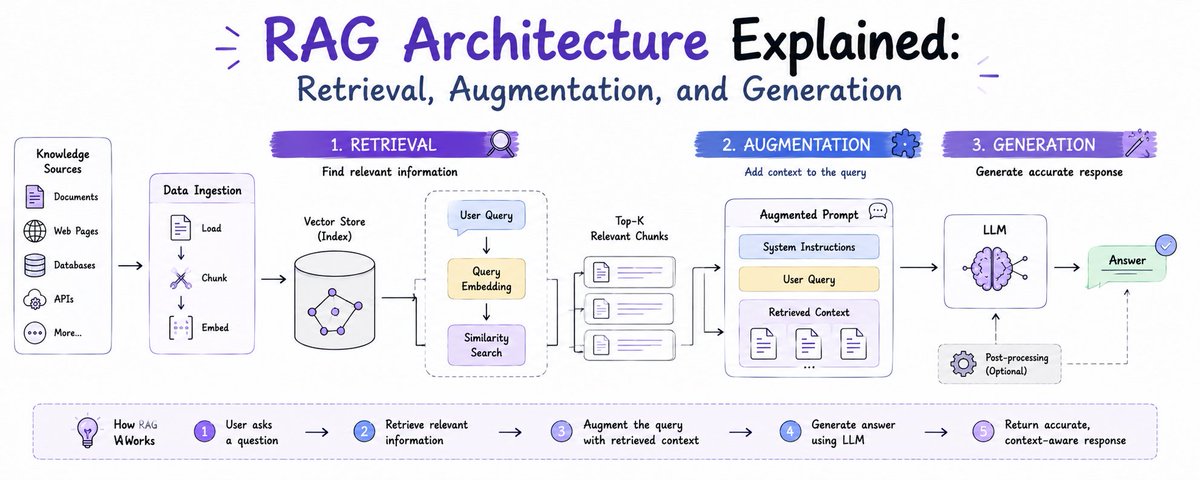
This is exactly what Retrieval-Augmented Generation (RAG) does. RAG is the architectural pattern that grounds every answer in external, verifiable knowledge. It prevents hallucinations, provides exact source citations, and updates the AI's knowledge base in real-time without requiring a multimillion-dollar fine-tuning run.
In this deep dive, we are going to break down the complete architecture of a production-grade RAG system. We will dissect the offline indexing pipeline, map out the online query lifecycle step-by-step, explore the relational data model required to store this information, and finally, look at the live metrics you must monitor to ensure your system is actually working.
Let us build a system that tells the truth.
## 1. System Architecture: The Two Planes
A modern RAG system is not a single script. It is a distributed architecture split into two entirely separate domains: the Knowledge Plane (Offline Indexing) and the Runtime Plane (Online Answering).
You can think of this like a massive library. The Knowledge Plane is the librarian constantly reading new books, categorizing them, and placing them on the correct shelves. The Runtime Plane is the desk clerk who takes your question, runs to the shelf, grabs the right book, and reads you the exact paragraph you need.
The Knowledge Plane (Offline Indexing)
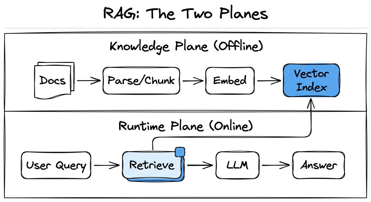
The Knowledge Plane is responsible for taking your messy, unstructured data and turning it into a format that a machine can search mathematically. This operates asynchronously, running in the background as batch jobs or scheduled CRON tasks.
1. The Sources: Data comes from everywhere. In a production system, your sources might include PDF manuals, Google Drive documents, raw SQL rows from your product database, or HTML from web crawls. This data is messy, heavily formatted, and completely unreadable to a vector engine in its raw state.
2. The Ingest Pipeline (Parse - Chunk - Embed): When a new document enters the system, it goes through a strict three-step pipeline:
- Parse: The system strips away the formatting. It removes HTML tags, extracts text from PDFs, and converts everything into raw, clean strings.
- Chunk: You cannot feed an entire 500-page manual into an LLM context window, nor can you search it effectively. The text is chopped into smaller, overlapping segments called "chunks." A standard chunk size might be 512 or 1024 tokens. We overlap these chunks slightly (e.g., by 50 tokens) so that if a crucial sentence spans the border of two chunks, the context is not lost.
- Embed: This is where the magic happens. The system passes each chunk of text through an embedding model (like OpenAI's text-embedding-3 or an open-source alternative). The model translates the text into a massive array of numbers. Specifically, it encodes the semantic meaning of the chunk into a 768-dimensional (768-D) vector. In 768-D space, concepts that mean the same thing are physically grouped closer together.
3. The Vector Index: Once the chunks are converted into 768-D vectors, they are batch-written into a Vector Database. However, storing them is not enough; they must be indexed for rapid searching. Production systems use algorithms like HNSW (Hierarchical Navigable Small World) or IVF (Inverted File Index) for Approximate Nearest Neighbor (ANN) search. These indexes organize the vectors so that when a user asks a question, the database does not have to scan every single chunk - it can instantly navigate to the correct "neighborhood" of data.
The Runtime Plane (Online Answering)
While the Knowledge Plane works in the background, the Runtime Plane is highly active, user-facing, and entirely latency-dependent. Every millisecond counts here. A production target for the read path is typically sub-300ms p95 latency.
1. User Query (Text In): The user types a question into the chat interface. For example: "What is our remote work policy?"
2. Retrieve and Rerank: The system takes that text, instantly embeds it into a 768-D vector, and fires it at the Vector Index. The index returns the Top-K (e.g., the top 5) most mathematically similar document chunks based on Cosine Similarity.
3. LLM Generator (Context In): The retrieved chunks of text are glued together alongside the user's original query and a strict system prompt. This massive block of context is passed into the generative LLM.
4. Answer and Cites (Sources Out): Because the LLM now has the exact text from the employee handbook sitting in its context window, it generates a perfectly accurate answer and attaches inline citations pointing directly to the source chunks.
## 2. The Query Lifecycle: A Step-by-Step Breakdown
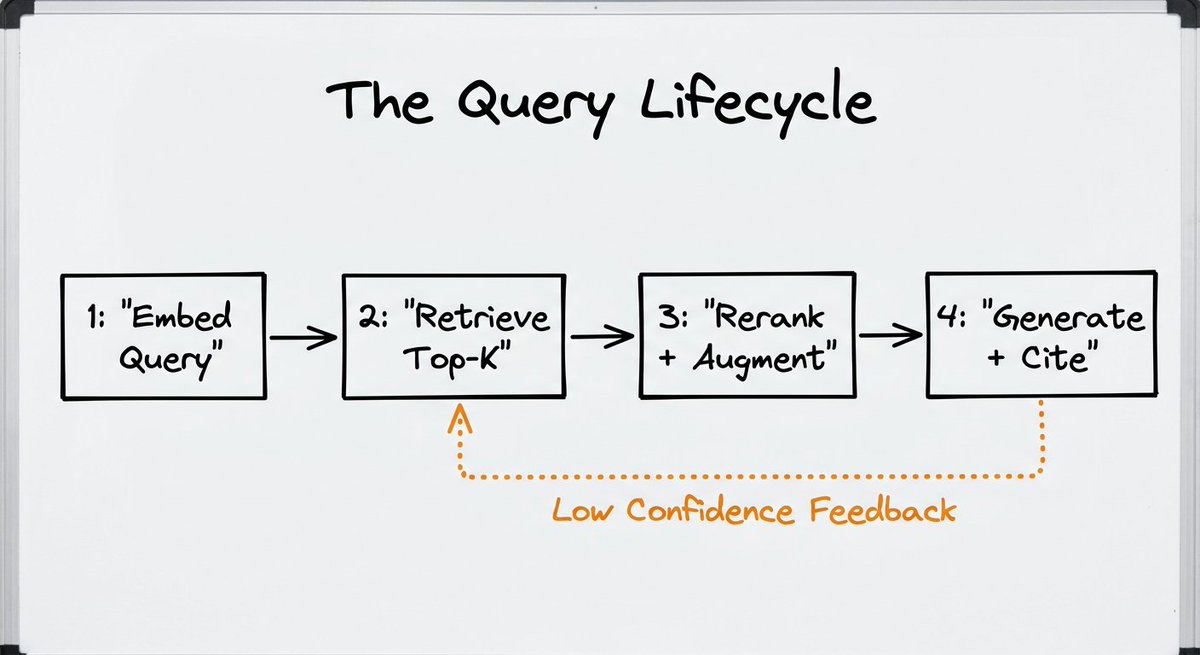
Let us zoom in on the Runtime Plane and look at the exact control flow of a single query. Every query that hits a RAG system runs the exact same four steps. It is a predictable forward pass with a critical feedback edge.
Step 01: Embed the Query
Before the system can find the answer, it must understand the question mathematically. When the user asks, "How do I reset my VPN password?", the system passes this raw text into the exact same embedding model used in the Knowledge Plane.
The question is encoded into a 768-D vector. This vector does not represent the exact keywords; it represents the intent and semantics of the question. This means the system can find documents that talk about "recovering network access credentials" even if the document never explicitly uses the words "reset," "VPN," or "password."
Step 02: Retrieve Top-K
The query vector is sent to the Vector Index as a search request. The database executes an Approximate Nearest Neighbor (ANN) search.
It calculates the Cosine Similarity between the query vector and millions of document chunk vectors. Cosine similarity measures the angle between two vectors; the smaller the angle, the closer the semantic meaning. The database returns the nearest chunks - usually defined as "Top-K" (e.g., K=5).
At this stage, you have the 5 most relevant paragraphs of text from your entire company database.
Step 03: Rerank and Augment
Vector search is incredibly fast, but it is not perfectly precise. Sometimes, the 4th returned chunk is actually more relevant to the user's specific question than the 1st returned chunk.
To fix this, advanced RAG architectures implement a "Reranker." The system takes the Top-K chunks and scores them again using a more computationally heavy model (like a Cross-Encoder). This reranker re-orders the chunks based on absolute relevance.
Once reranked, we hit the "Augment" phase. The system injects this highly relevant context directly into the LLM's prompt.
Here is what that augmented prompt looks like in code:
```
SYSTEM PROMPT:
You are a helpful company assistant.
Answer the user's query using ONLY the provided context.
If the answer is not in the context, you must state "I do not know."
Always cite the source document ID.
CONTEXT:
[Doc_142]: The IT portal for recovering network credentials is at vpn.company.internal.
[Doc_199]: Password resets require two-factor authentication via the mobile app.
USER QUERY:
How do I reset my VPN password?
```
Step 4: Generate and Cite
The LLM processes the massive augmented prompt. Because it is strictly constrained by the instructions, it does not hallucinate. It reads the context, synthesizes the information, and generates the final response.
Crucially, it provides inline source citations. The output looks like this: "To reset your VPN password, navigate to [vpn.company](//vpn.company).internal [Doc_142]. Please note that you will need to complete two-factor authentication using your mobile app [Doc_199]."
The Feedback Loop (Self-Correction)
What happens if the Vector Index returns irrelevant chunks? If the LLM looks at the context and realizes the answer simply is not there, the system will trigger a feedback edge.
When the LLM confidence is low, it emits a failure flag. The system catches this flag and triggers a Re-query. It might use an LLM to rewrite the user's original query into a broader search term, embed the new query, and try the pipeline again. This internal loop ensures the user never sees a hallucination.
## 3. The Relational Data Model
RAG is fundamentally a data engineering problem. If you do not map your entity relationships correctly, your system will be impossible to debug, and your UI will be incapable of showing users the original source files.
Let us break down the exact database schema required to operate a production RAG system, looking at the entity relations and cardinality.
Users and Queries
Everything starts with the user.
- USER Table: Contains user_id (Primary Key) and name.
- QUERY Table: Contains query_id (Primary Key), the user_id (Foreign Key), and the raw text of their question. The relationship here is One-to-Many (1:N). One user can submit many queries.
Documents, Chunks, and Embeddings
This is the core of the Knowledge Plane.
- DOCUMENT Table: Contains doc_id (Primary Key), the url, and the source type (e.g., PDF or Confluence).
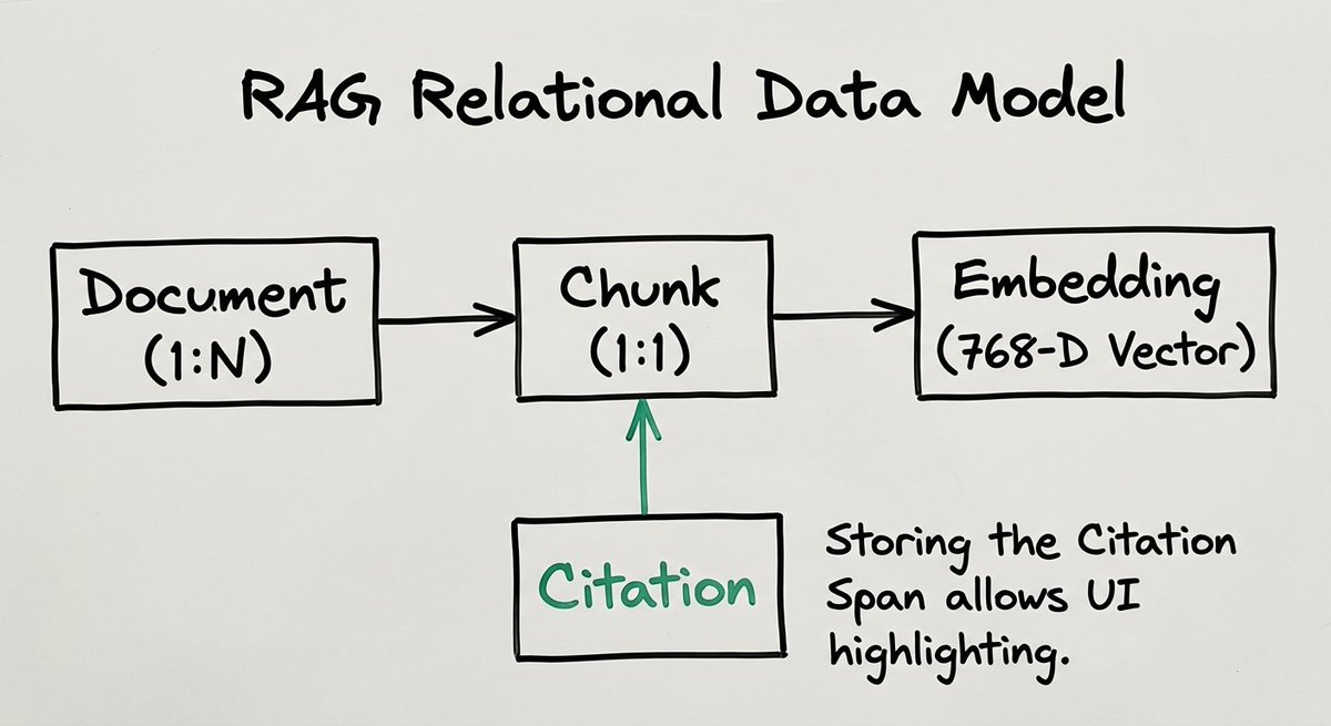
- CHUNK Table: Contains chunk_id (Primary Key), the doc_id (Foreign Key), and the actual raw text of the chunk. The relationship is 1:N. One document contains many chunks.
- EMBEDDING Table: Contains embed_id (Primary Key), the chunk_id (Foreign Key), and the actual vector[768] array. The relationship here is One-to-One (1:1). Every text chunk has exactly one mathematical vector representation.
Retrievals, Answers, and Citations
This is where the Runtime Plane data is logged for telemetry and UI rendering.
- RETRIEVAL Table: This is a mapping table containing query_id and chunk_id. It logs the score (the cosine similarity metric). The relationship is Many-to-Many (M:N). One query fetches many chunks, and one chunk can be fetched by many queries.
- ANSWER Table: Contains answer_id (Primary Key), the query_id (Foreign Key), and the final generated text.
- CITATION Table: Contains the answer_id (Foreign Key), the chunk_id (Foreign Key), and the span (the exact character start and end index in the answer where the citation occurs). The relationship is 1:N. One answer contains many citations.
Storing the span in the Citation table is incredibly important. When you render the answer in your React frontend, the span tells the UI exactly which words to highlight in yellow so the user can click them and view the original chunk.
## 4. Live Metrics: Measuring RAG Quality
You cannot manage what you cannot measure. Because RAG systems are non-deterministic, you must rely on advanced statistical telemetry to ensure your system is performing well.
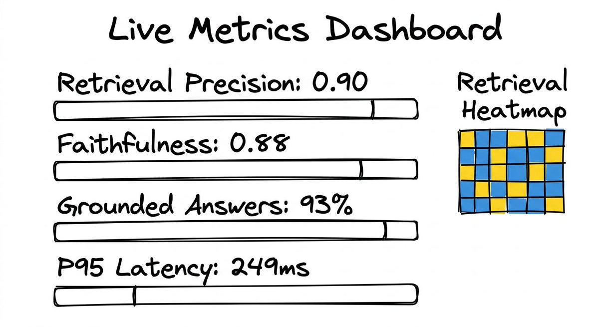
A standard production dashboard tracks four critical live metrics:
1. Retrieval Precision
Target Benchmark: ~0.90 Retrieval precision measures whether the Vector Index is actually fetching the right data. If a user asks about health insurance, and the system fetches chunks about office parking policies, your retrieval precision is zero.
This is measured by looking at the Top-K chunks returned and calculating what percentage of them were actually highly relevant to the query. If your precision drops, it means your embedding model is weak, or your chunk sizes are too large, resulting in diluted semantic meaning.
2. Faithfulness Score
Target Benchmark: ~0.88 This metric is entirely focused on the LLM Generator. Faithfulness evaluates whether the final generated answer is strictly tied to the retrieved context.
If the LLM ignores the context and injects its own outside knowledge, it is "unfaithful" to the prompt. An unfaithful model is a massive legal and compliance risk in an enterprise setting. You measure this by using an independent "Judge LLM" that reads the answer, reads the chunks, and flags any claims that cannot be traced back to the source.
3. Grounded Answers
Target Benchmark: ~93% This metric tracks the absolute percentage of queries where the system successfully generated an answer backed by citations.
If this number drops, it means one of two things: either your vector database is empty and lacking the necessary documents, or your users are asking questions outside the scope of the system. Tracking grounded answers helps your data engineering team identify "knowledge gaps" in the pipeline.
4. P95 Latency (Read Path)
Target Benchmark: ~249 ms Speed is a feature. P95 latency means that 95% of all queries are processed in under this time threshold. A standard benchmark for a highly optimized RAG system is roughly 250 to 300 milliseconds.
If your latency spikes, the user experience degrades into a frustrating loading spinner. High latency is usually caused by the Reranking step (which is computationally expensive) or by selecting an LLM generator that is too large and slow for the task.
The Retrieval Heatmap
Beyond hard numbers, operators use Retrieval Heatmaps to visualize Top-K similarity per query. A heatmap displays rows of blocks, where each block represents a retrieved chunk. Dark blue blocks indicate high cosine similarity, while yellow or orange blocks indicate low confidence.
If your heatmap is consistently showing low-confidence retrievals, it visually signals that the system is struggling to find exact matches for user queries, prompting the engineering team to overhaul the ingest pipeline.
## Advanced Chunking Strategies
While the basic pipeline describes chopping text into static 512-token blocks, production systems require much more nuance. If you blindly slice a document every 500 tokens, you will inevitably cut a crucial paragraph in half, destroying its semantic meaning before it even reaches the embedding model.
To solve this, data engineers use semantic chunking. Instead of splitting by token count, the parser uses a natural language processor to identify sentence boundaries, paragraph breaks, and even markdown headers.
Parent-Child Chunking
Another advanced technique is Parent-Child Chunking (often called Hierarchical Indexing). In this model, you chunk the document twice. First, you create large "Parent" chunks (e.g., 2000 tokens) that capture broad context. Then, you break those parents down into smaller "Child" chunks (e.g., 250 tokens) and embed the children into the Vector Index.
When a user searches the index, the algorithm matches against the specific, highly-focused Child chunk. But instead of returning the Child to the LLM, the system retrieves the entire Parent chunk attached to it. This guarantees that the LLM receives the highly specific answer along with the broad surrounding context, virtually eliminating hallucination risks caused by missing information.
## Cross-Encoders vs. Bi-Encoders
In Step 03 of the Query Lifecycle, we discussed Reranking. It is crucial to understand the difference between the two models at play here.
The initial retrieval (Step 02) uses a Bi-Encoder. A Bi-Encoder processes the user's query and the document chunks independently, turns them both into 768-D vectors, and calculates the angle between them. It is incredibly fast, allowing you to search millions of documents in milliseconds. However, it lacks deep contextual understanding because it never looks at the query and the document at the same time.
The reranker (Step 03) uses a Cross-Encoder. A Cross-Encoder does not output vectors. Instead, it takes the user's query and a single retrieved document chunk, feeds them into the neural network together, and outputs a highly accurate relevance score from 0 to 1.
Because the Cross-Encoder processes both texts simultaneously, it understands deep linguistic nuances and complex phrasing that the Bi-Encoder misses. You cannot run a Cross-Encoder over your entire 10-million document database - it would take hours. But running it over the Top-100 results returned by the Bi-Encoder takes only a few milliseconds, giving you the perfect blend of blazing speed and pinpoint accuracy.
## 5. Building the Pipeline (Technical Implementation)
To pull this all together, let us look at a simplified, highly practical Python implementation of the Runtime Plane using standard modern tooling.
This script demonstrates how you embed a query, retrieve the top chunks, construct the augmented prompt, and generate the cited answer.
```
import numpy as np
from typing import List, Dict
# Simulated client libraries
import vector_db_client
import llm_client
def execute_rag_pipeline(user_query: str) -> str:
print(f"--- INITIATING RAG PIPELINE ---")
print(f"User Query: {user_query}")
# Step 1: Embed Query (Encode as 768-D Vector)
query_vector = llm_client.embed_text(
text=user_query,
model="text-embedding-3-small"
)
# Step 2: Retrieve Top-K from HNSW Index
top_k_results = vector_db_client.search(
collection="company_knowledge_base",
vector=query_vector,
top_k=3,
metric="cosine_similarity"
)
# Check if retrieval confidence is high enough
if top_k_results[0].score < 0.70:
return "System Notification: Confidence too low. Re-query required."
# Step 3: Augment Prompt
formatted_context = ""
for doc in top_k_results:
formatted_context += f"\n[Doc_{doc.id}]: {doc.text}"
system_prompt = "You are a strict technical assistant. Answer using ONLY the provided context. Cite sources using [Doc_ID].\nCONTEXT:\n" + formatted_context
# Step 4: Generate and Cite
final_answer = llm_client.generate(
system=system_prompt,
user_message=user_query,
model="claude-3-haiku-20240307",
temperature=0.0 # Absolute zero for strict determinism
)
return final_answer
```
This simple script captures the entire essence of the RAG architecture. It creates the semantic vector, searches the mathematical space, constructs the strict context boundaries, and forces the LLM to act as a grounded synthesizer rather than a creative hallucinator.
## The Future is Agentic
Retrieval-Augmented Generation is no longer an experimental feature; it is the absolute baseline requirement for any production AI system.
But the architecture we just mapped out - the linear step-by-step flow from embedding to generation - is just the beginning. The industry is rapidly moving toward "Agentic RAG."
In an Agentic RAG system, the pipeline is not a strict forward pass. The LLM acts as an autonomous worker. It retrieves a document, reads it, realizes the document only contains half the answer, actively formulates a new search query, retrieves a second document, and synthesizes them both before replying to the user.
But before you can build an agent that navigates documents autonomously, you must perfectly engineer the foundational pipes. You need a fast Ingest Pipeline, a perfectly mapped Relational Data Model, and a sub-300ms Vector Index.
Ground your answers. Cite your sources. Build systems you can trust.
Subscribe to [ByteBuilders](https://bytebuilders.beehiiv.com/subscribe) and get the next deep dive in your inbox:
## 相关链接
- [Vikas gupta](https://x.com/vicky_grok)
- [@vicky_grok](https://x.com/vicky_grok)
- [1.4K](https://x.com/vicky_grok/status/2090064227570766226/analytics)
- [vpn.company](https://vpn.company/)
- [ByteBuilders](https://bytebuilders.beehiiv.com/subscribe)
- [Upgrade to Premium](https://x.com/i/premium_sign_up)
- [9:11 PM · Aug 19, 2026](https://x.com/vicky_grok/status/2090064227570766226)
- [1,489 Views](https://x.com/vicky_grok/status/2090064227570766226/analytics)
---
*导出时间: 2026/8/20 09:35:13*
---
## 中文翻译
# RAG架构详解:检索、增强与生成
**作者**: Vikas gupta
**日期**: 2026-08-19T13:11:58.000Z
**来源**: [https://x.com/vicky_grok/status/2090064227570766226](https://x.com/vicky_grok/status/2090064227570766226)
---

如果你最近花过时间使用AI构建应用,你很可能已经遇到了大型语言模型(LLM)的根本性局限:它们不了解你的私有数据。
你可以让LLM写一首诗、解释量子物理,或者格式化一段JSON,它会表现得非常出色。但如果你问它公司第三季度的营收现状,或者内部员工手册中的具体故障排除步骤,它要么拒绝回答,要么更糟糕——它会编造一个听起来非常自信的谎言。
LLM在完成训练的那一刻就被冻结在时间里了。它们只知道公开数据。要让LLM在企业环境中发挥作用,你必须给它一个“记忆”。
这正是检索增强生成(RAG)所做的事情。RAG是一种架构模式,它将每一个答案都锚定在外部、可验证的知识之上。它防止幻觉,提供精确的来源引用,并实时更新AI的知识库,而无需进行耗资数百万美元的微调。
在本次深度解析中,我们将完整拆解一个生产级RAG系统的架构。我们将剖析离线索引管道,逐步梳理在线查询生命周期,探索存储这些信息所需的关系数据模型,最后,看看你必须监控的实时指标,以确保系统真正在正常工作。
让我们构建一个说真话的系统。
## 1. 系统架构:两个平面
一个现代RAG系统不是单个脚本。它是一个分布式架构,分为两个完全独立的领域:知识平面(离线索引)和运行时平面(在线回答)。
你可以把它想象成一个巨大的图书馆。知识平面是图书管理员,不断阅读新书、分类并将它们放到正确的书架上。运行时平面是前台服务员,他接过你的问题,跑到书架前,拿起正确的书,读给你听你需要的准确段落。
知识平面(离线索引)

知识平面负责接收你杂乱无章的非结构化数据,并将其转换为机器可以数学化搜索的格式。这以异步方式运行,作为批处理作业或定时CRON任务在后台执行。
1. **数据源**:数据来自各个地方。在生产系统中,你的数据源可能包括PDF手册、Google Drive文档、产品数据库中的原始SQL行,或来自网络爬虫的HTML。这些数据是杂乱的、格式繁重的,在原始状态下对向量引擎完全不可读。
2. **摄取管道(解析-分块-嵌入)**:当新文档进入系统时,它要经过严格的三步管道:
- **解析**:系统剥离格式。它移除HTML标签,从PDF中提取文本,并将所有内容转换为干净的原始字符串。
- **分块**:你不能把一本500页的手册全部塞进LLM的上下文窗口,也无法有效地搜索它。文本被切成更小的、有重叠的片段,称为“块”。标准块大小可能是512或1024个token。我们会让这些块有轻微的重叠(例如,重叠50个token),这样如果一句关键的话跨越了两个块的边界,上下文也不会丢失。
- **嵌入**:这是魔法发生的地方。系统将每个文本块通过嵌入模型(如OpenAI的text-embedding-3或开源替代方案)。模型将文本转换为一个巨大的数字数组。具体来说,它将块的语义含义编码为一个768维(768-D)向量。在768维空间中,含义相同的概念在物理上会被分组得更近。
3. **向量索引**:一旦块被转换为768维向量,它们就会被批量写入向量数据库。然而,仅仅存储是不够的;它们必须被索引以便快速搜索。生产系统使用HNSW(分层可导航小世界)或IVF(倒排文件索引)等算法进行近似最近邻(ANN)搜索。这些索引组织向量,使得当用户提问时,数据库不必扫描每一个块——它可以立即导航到正确的数据“邻域”。
运行时平面(在线回答)
当知识平面在后台工作时,运行时平面是高度活跃的、面向用户的,并且完全依赖延迟。这里每一毫秒都很重要。生产环境的读取路径目标通常是p95延迟低于300毫秒。
1. **用户查询(文本输入)**:用户在聊天界面中输入问题。例如:“我们的远程工作政策是什么?”
2. **检索与重排序**:系统获取该文本,立即将其嵌入为768维向量,并将其发送到向量索引。索引基于余弦相似度返回Top-K(例如,最相似的5个)文档块。
3. **LLM生成器(上下文输入)**:检索到的文本块与用户的原始查询和严格的系统提示词粘合在一起。这一大块上下文被传入生成式LLM。
4. **回答与引用(来源输出)**:因为LLM的上下文窗口中现在有了员工手册中的确切文本,它会生成一个完全准确的答案,并附上直接指向源块的内联引用。
## 2. 查询生命周期:逐步拆解
让我们放大运行时平面,看看单个查询的确切控制流。每个到达RAG系统的查询都运行完全相同的四个步骤。这是一个可预测的前向传递,带有一个关键的反馈边。

步骤01:嵌入查询
在系统找到答案之前,它必须在数学上理解问题。当用户问“我如何重置我的VPN密码?”时,系统将这个原始文本传入与知识平面中使用的完全相同的嵌入模型。
该问题被编码为一个768维向量。这个向量不代表确切的关键词;它代表问题的意图和语义。这意味着系统可以找到讨论“恢复网络访问凭据”的文档,即使文档从未明确使用“重置”、“VPN”或“密码”这些词。
步骤02:检索Top-K
查询向量作为搜索请求被发送到向量索引。数据库执行近似最近邻(ANN)搜索。
它计算查询向量与数百万个文档块向量之间的余弦相似度。余弦相似度衡量两个向量之间的角度;角度越小,语义含义越接近。数据库返回最近的块——通常定义为“Top-K”(例如,K=5)。
在这个阶段,你得到了整个公司数据库中最相关的5个文本段落。
步骤03:重排序与增强
向量搜索非常快,但并非完美精确。有时,返回的第4个块实际上比返回的第1个块与用户的具体问题更相关。
为了解决这个问题,高级RAG架构实现了“重排序器”。系统获取Top-K块,并使用一个计算量更大的模型(如交叉编码器)再次对它们进行评分。这个重排序器根据绝对相关性重新排列块的顺序。
重排序完成后,我们进入“增强”阶段。系统将高度相关的上下文直接注入LLM的提示词中。
以下是增强后的提示词在代码中的样子:
```
系统提示词:
你是一个乐于助人的公司助理。
仅使用提供的上下文回答用户的查询。
如果答案不在上下文中,你必须声明“我不知道”。
始终引用源文档ID。
上下文:
[Doc_142]:用于恢复网络凭据的IT门户位于 vpn.company.internal。
[Doc_199]:密码重置需要通过移动应用进行双重身份验证。
用户查询:
我如何重置我的VPN密码?
```
步骤4:生成与引用
LLM处理这个庞大的增强提示词。因为它受到指令的严格约束,它不会产生幻觉。它阅读上下文,综合信息,并生成最终响应。
至关重要的是,它提供内联来源引用。输出看起来像这样:“要重置你的VPN密码,请导航到 [vpn.company](//vpn.company).internal [Doc_142]。请注意,你需要使用移动应用完成双重身份验证 [Doc_199]。”
反馈循环(自我纠正)
如果向量索引返回了不相关的块怎么办?如果LLM查看上下文并意识到答案根本不在其中,系统将触发一个反馈边。
当LLM置信度较低时,它会发出一个失败标志。系统捕获此标志并触发重新查询。它可能使用LLM将用户的原始查询重写为更广泛的搜索词,嵌入新查询,然后再次尝试管道。这个内部循环确保用户永远不会看到幻觉。
## 3. 关系数据模型
RAG本质上是一个数据工程问题。如果你没有正确映射实体关系,你的系统将无法调试,你的UI也将无法向用户展示原始源文件。
让我们分解运行生产级RAG系统所需的确切数据库模式,查看实体关系和基数。
用户与查询
一切从用户开始。
- **USER表**:包含user_id(主键)和name。
- **QUERY表**:包含query_id(主键)、user_id(外键)以及用户问题的原始文本。这里的关系是一对多(1:N)。一个用户可以提交多个查询。

文档、块与嵌入
这是知识平面的核心。
- **DOCUMENT表**:包含doc_id(主键)、url和源类型(例如,PDF或Confluence)。
- **CHUNK表**:包含chunk_id(主键)、doc_id(外键)以及块的实际原始文本。关系是1:N。一个文档包含多个块。
- **EMBEDDING表**:包含embed_id(主键)、chunk_id(外键)以及实际的vector[768]数组。这里的关系是一对一(1:1)。每个文本块恰好有一个数学向量表示。
检索、答案与引用
这是运行时平面数据被记录用于遥测和UI渲染的地方。
- **RETRIEVAL表**:这是一个映射表,包含query_id和chunk_id。它记录得分(余弦相似度指标)。关系是多对多(M:N)。一个查询获取多个块,一个块可以被多个查询获取。
- **ANSWER表**:包含answer_id(主键)、query_id(外键)以及最终生成的文本。
- **CITATION表**:包含answer_id(外键)、chunk_id(外键)以及span(答案中引用发生的精确字符起始和结束索引)。关系是1:N。一个答案包含多个引用。
在引用表中存储span非常重要。当你在React前端渲染答案时,span告诉UI确切要突出显示哪些词,以便用户可以点击它们并查看原始块。
## 4. 实时指标:衡量RAG质量
你无法管理无法衡量的东西。因为RAG系统是非确定性的,你必须依赖先进的统计遥测来确保系统运行良好。
一个标准的生产仪表板跟踪四个关键的实时指标:

1. **检索精确度**
目标基准:约0.90 检索精确度衡量向量索引是否实际获取了正确的数据。如果用户询问健康保险,而系统获取了关于办公室停车政策的块,那么你的检索精确度就是零。
这是通过查看返回的Top-K块并计算其中实际与查询高度相关的百分比来衡量的。如果你的精确度下降,意味着你的嵌入模型较弱,或者你的块大小太大,导致语义含义被稀释。
2. **忠实度得分**
目标基准:约0.88 这个指标完全聚焦于LLM生成器。忠实度评估最终生成的答案是否严格与检索到的上下文相关联。
如果LLM忽略上下文并注入自己的外部知识,那么它对提示词就是“不忠实的”。在企业环境中,不忠实的模型是巨大的法律和合规风险。你通过使用一个独立的“裁判LLM”来测量这一点,它阅读答案、阅读块,并标记任何无法追溯到来源的声明。
3. **有依据的答案**
目标基准:约93% 这个指标跟踪系统成功生成有引用支持的答案的查询绝对百分比。
如果这个数字下降,意味着两种情况之一:要么你的向量数据库为空,缺少必要的文档;要么你的用户在询问系统范围之外的问题。跟踪有依据的答案有助于你的数据工程团队识别管道中的“知识缺口”。
4. **P95延迟(读取路径)**
目标基准:约249毫秒 速度是一项功能。P95延迟意味着95%的查询在此时间阈值内处理完成。一个高度优化的RAG系统的标准基准大约是250到300毫秒。
如果你的延迟飙升,用户体验就会退化为令人沮丧的加载转圈。高延迟通常由重排序步骤(计算成本高)或选择了对于任务来说过大过慢的LLM生成器引起。
检索热力图
除了硬性数字之外,运维人员使用检索热力图来可视化每次查询的Top-K相似度。热力图显示行块,每个块代表一个检索到的块。深蓝色块表示高余弦相似度,而黄色或橙色块表示低置信度。
如果你的热力图持续显示低置信度检索,这直观地表明系统难以找到用户查询的精确匹配,促使工程团队彻底检修摄取管道。
## 高级分块策略
虽然基本管道描述的是将文本切成静态的512-token块,但生产系统需要更多的精细度。如果你盲目地每500个token切一次文档,你不可避免地会把一个关键段落切成两半,在它到达嵌入模型之前就破坏了其语义含义。
为了解决这个问题,数据工程师使用语义分块。解析器不是按token数分割,而是使用自然语言处理器来识别句子边界、段落分隔符,甚至Markdown标题。
父子分块
另一种高级技术是父子分块(通常称为分层索引)。在这种模型中,你对文档进行两次分块。首先,你创建大的“父”块(例如,2000个token)来捕获广泛的上下文。然后,你将父块分解为更小的“子”块(例如,250个token),并将子块嵌入到向量索引中。
当用户搜索索引时,算法匹配特定的、高度聚焦的子块。但系统不是将子块返回给LLM,而是检索附加在其上的整个父块。这保证了LLM接收到高度具体的答案以及广泛的周围上下文,几乎消除了因信息缺失导致的幻觉风险。
## 交叉编码器与双编码器
在查询生命周期的步骤03中,我们讨论了重排序。理解这里两个模型之间的区别至关重要。
初始检索(步骤02)使用双编码器。双编码器独立处理用户的查询和文档块,将它们都转换为768维向量,并计算它们之间的角度。它非常快,让你可以在毫秒内搜索数百万个文档。然而,它缺乏深层的上下文理解,因为它从不同时查看查询和文档。
重排序器(步骤03)使用交叉编码器。交叉编码器不输出向量。相反,它获取用户的查询和一个检索到的文档块,将它们一起输入神经网络,并输出一个从0到1的高度准确的相关性得分。
因为交叉编码器同时处理两个文本,它理解了双编码器遗漏的深层语言细微差别和复杂措辞。你不能在拥有1000万文档的整个数据库上运行交叉编码器——那需要数小时。但在双编码器返回的Top-100结果上运行它只需要几毫秒,让你获得极速与精准的完美结合。
## 5. 构建管道(技术实现)
为了把所有内容整合起来,让我们看一个使用标准现代工具实现的、简化且高度实用的运行时平面Python实现。
这个脚本演示了如何嵌入查询、检索顶部块、构建增强提示词并生成带引用的答案。
```
import numpy as np
from typing import List, Dict
# 模拟客户端库
import vector_db_client
import llm_client
def execute_rag_pipeline(user_query: str) -> str:
print(f"--- 启动RAG管道 ---")
print(f"用户查询: {user_query}")
# 步骤 1: 嵌入查询(编码为768维向量)
query_vector = llm_client.embed_text(
text=user_query,
model="text-embedding-3-small"
)
# 步骤 2: 从HNSW索引检索Top-K
top_k_results = vector_db_client.search(
collection="company_knowledge_base",
vector=query_vector,
top_k=3,
metric="cosine_similarity"
)
# 检查检索置信度是否足够高
if top_k_results[0].score < 0.70:
return "系统通知:置信度过低。需要重新查询。"
# 步骤 3: 增强提示词
formatted_context = ""
for doc in top_k_results:
formatted_context += f"\n[Doc_{doc.id}]: {doc.text}"
system_prompt = "你是一个严格的技术助理。仅使用提供的上下文回答。使用[Doc_ID]引用来源。\n上下文:\n" + formatted_context
# 步骤 4: 生成与引用
final_answer = llm_client.generate(
system=system_prompt,
user_message=user_query,
model="claude-3-haiku-20240307",
temperature=0.0 # 绝对零度以确保严格确定性
)
return final_answer
```
这个简单的脚本捕获了RAG架构的全部精髓。它创建语义向量,搜索数学空间,构建严格的上下文边界,并迫使LLM充当有依据的综合者,而不是创造性的幻觉者。
## 未来是智能体化的
检索增强生成不再是一个实验性功能;它是任何生产级AI系统的绝对基线要求。
但我们刚刚描绘的架构——从嵌入到生成的线性逐步流程——仅仅是个开始。行业正在迅速向“智能体RAG”发展。
在智能体RAG系统中,管道不是严格的前向传递。LLM充当自主工作者。它检索一个文档,阅读它,意识到文档只包含答案的一半,主动制定新的搜索查询,检索第二个文档,并在回复用户之前综合两者。
但在你能构建一个自主导航文档的智能体之前,你必须完美地工程化基础管道。你需要一个快速的摄取管道、一个完美映射的关系数据模型,以及一个亚300毫秒的向量索引。
让你的答案有依据。引用你的来源。构建你可以信任的系统。
订阅 [ByteBuilders](https://bytebuilders.beehiiv.com/subscribe),让下一篇深度解析直接进入你的收件箱:
## 相关链接
- [Vikas gupta](https://x.com/vicky_grok)
- [@vicky_grok](https://x.com/vicky_grok)
- [1.4K](https://x.com/vicky_grok/status/2090064227570766226/analytics)
- [vpn.company](https://vpn.company/)
- [ByteBuilders](https://bytebuilders.beehiiv.com/subscribe)
- [Upgrade to Premium](https://x.com/i/premium_sign_up)
- [9:11 PM · Aug 19, 2026](https://x.com/vicky_grok/status/2090064227570766226)
- [1,489 Views](https://x.com/vicky_grok/status/2090064227570766226/analytics)
---
*导出时间: 2026/8/20 09:35:13*