# From Prompt to Response Inside an LLM: A Visual Step-by-Step Journey With Code
**作者**: Vikas gupta
**日期**: 2026-08-09T04:57:29.000Z
**来源**: [https://x.com/vicky_grok/status/2086315908344266782](https://x.com/vicky_grok/status/2086315908344266782)
---
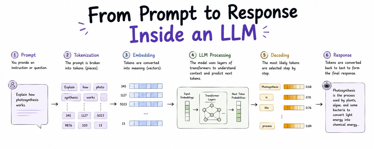
You type "Explain transformers like I am 12" and hit enter. 800 milliseconds later you get five paragraphs back.
In those 800 milliseconds, your 6 words turned into tokens, tokens turned into 12,288-dimensional vectors, those vectors passed through 96 layers of attention and feed-forward networks, interacted with a KV-cache that remembers previous tokens, became probabilities over 100,000 possible next words, were sampled with temperature and top-p, and were detokenized back into readable text.
Most explainers stop at "transformer magic." This article shows you every step with code you can run.
## Part 1: Step 1 - Tokenization - Your Text Is Not Text to the Model
LLMs do not read characters. They read tokens.
A token is a chunk of text the model learned during training. It can be a whole word like "response", a part like "prompt", or even a single character.
Why tokenize? To balance vocabulary size and sequence length. If you use characters, your sequence is too long. If you use whole words, vocabulary is too large and you cannot handle new words.
How BPE Works in 30 Seconds
Byte Pair Encoding starts with characters. It repeatedly merges the most frequent adjacent pair.
Example:
- Start: l o w _ l o w e r _ n e w e s t
- Most frequent pair: l o
- Merge: lo w _ lo w e r _ n e w e s t
- Next frequent: lo w -> low
- Continue until vocabulary size reached, say 100k merges.
Result: Common word "low" becomes one token. Rare word "lowermost" becomes low + er + most = 3 tokens.
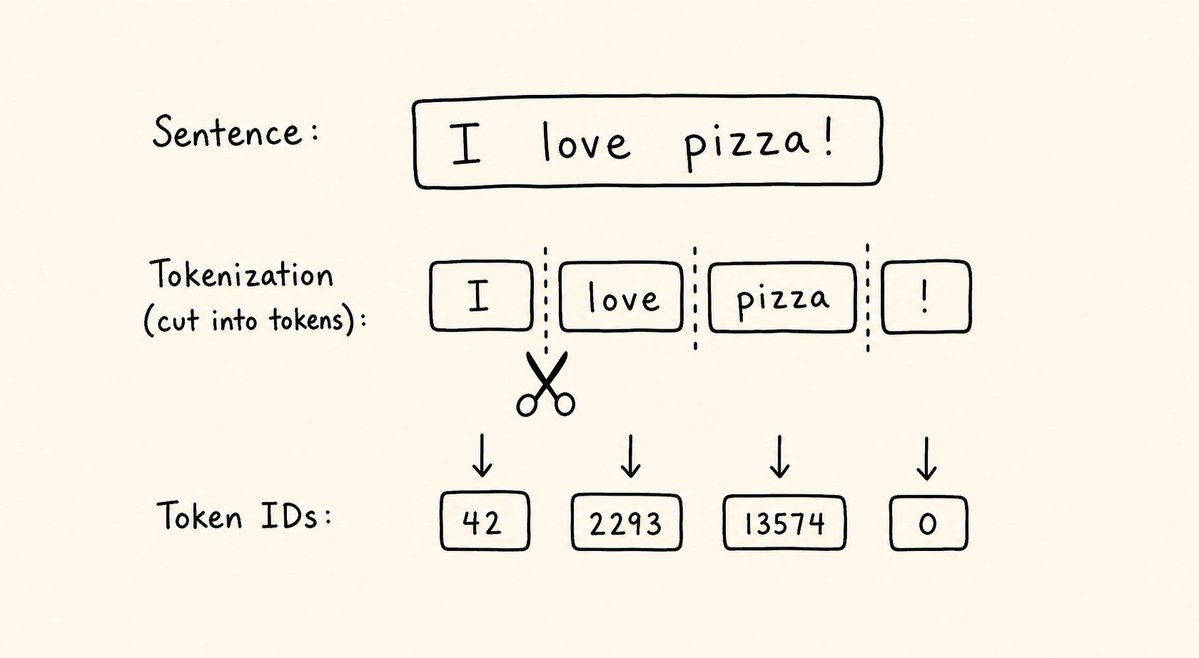
Code Example 1: See Tokenization Live With tiktoken
```
import tiktoken
# gpt-4o tokenizer cl100k_base is a good reference
enc = tiktoken.get_encoding("cl100k_base")
prompt = "From Prompt to Response Inside an LLM"
tokens = enc.encode(prompt)
decoded = [enc.decode([t]) for t in tokens]
print(f"Text: {prompt}")
print(f"Token IDs: {tokens}")
print(f"Decoded tokens: {decoded}")
print(f"Token count: {len(tokens)}")
# Output approx:
# Text: From Prompt to Response Inside an LLM
# Token IDs: [17346, 14508, 284, 24796, 2310, 260, 12382]
# Decoded tokens: ['From', ' Prompt', ' to', ' Response', ' Inside', ' an', ' LLM']
# Token count: 7
# Try longer
long_prompt = "From Prompt to Response Inside an LLM: A Visual Step-by-Step Journey"
print(enc.encode(long_prompt), len(enc.encode(long_prompt)))
# 14 tokens approx
# Why this matters: You pay per token, and context window is token count, not word count
```
Practical insight: " an LLM" is 2 tokens, but " an LLM." is 3 tokens because the period merges differently. Add a space at start and you save tokens for many models - " Prompt" is one token, "Prompt" at start of string can be different ID.
Table: Tokenization Examples (cl100k_base)
| Text | Tokens | Why |
| --- | --- | --- |
| Hello | 1 | Common word in vocab |
| Hello world | 2 | Space + word merged |
| HelloWorld | 2-3 | CamelCase splits |
| https://example.com | 4-6 | Symbols cause splits |
| 123456 | 2-3 | Numbers tokenized in chunks |
| | 3-6 | Emoji multi-token, expensive |
Rule: If you build RAG, chunk by tokens not characters. Use tiktoken to count.
Prompt Template:
> "Count tokens for this prompt [your prompt] using cl100k_base and suggest 2 shorter versions that keep meaning but use 20 percent fewer tokens. Explain which words are multi-token."
## Part 2: Step 2 - Embeddings and Positional Encoding - Turning IDs Into Meaning
After tokenization, each token ID looks up an embedding vector. Think of it as a coordinate in meaning space.
If vocab is 100k and embedding dimension is 4096 (like Llama 3 8B), embedding table is 100k x 4096 = 400M parameters alone.
token_id 17346 (From) -> [0.021, -0.134, 0.892, ..., 0.011] 4096 numbers.
But From at position 1 and From at position 10 should be treated differently because order matters. Self-attention has no built-in order. So we add positional encoding.
Two common types:
- Absolute positional encoding (original transformer): Sine and cosine waves added to embedding based on position index. Position 1 gets wave A, position 2 gets wave B.
- RoPE (Rotary Position Embedding - used by Llama 3, Mistral, GPT-4): Rotates embedding vector in complex space by angle proportional to position. Better for long context extrapolation.
Result after embedding + positional encoding: You have sequence of vectors [x1, x2, x3, ..., x7] each 4096-dim that knows both WHAT the token is and WHERE it is.
Code Example 2: Embedding Lookup with HuggingFace
```
from transformers import AutoTokenizer, AutoModel
import torch
tokenizer = AutoTokenizer.from_pretrained("meta-llama/Meta-Llama-3-8B-Instruct")
model = AutoModel.from_pretrained("meta-llama/Meta-Llama-3-8B-Instruct")
prompt = "From Prompt to Response"
inputs = tokenizer(prompt, return_tensors="pt")
# inputs.input_ids = token ids [1, 17346, ...]
# Embedding layer only
embeddings = model.model.embed_tokens(inputs.input_ids)
print(embeddings.shape) # torch.Size([1, 5, 4096]) = batch, seq_len, dim
# Compare cosine similarity of "prompt" and "response" embeddings
import torch.nn.functional as F
sim = F.cosine_similarity(embeddings[0][1], embeddings[0][3], dim=0)
print(f"Similarity prompt vs response in this context: {sim:.3f}")
```
In context, "prompt" and "response" are not far because they co-occur often in instruction data. Embedding is contextual later after attention, but starts with static lookup.
## Part 3: Step 3 - Self-Attention - The Core Magic You Can Build Intuition For
This is where meaning is created.
Goal: For each token, figure out which other tokens matter for understanding it.
Sentence: "The bank by the river banked money."
The first "bank" should attend to "river", the second "bank" should attend to "money" and "banked". Same word, different meaning based on context.
Self-Attention in 4 Steps (No Math Overload)
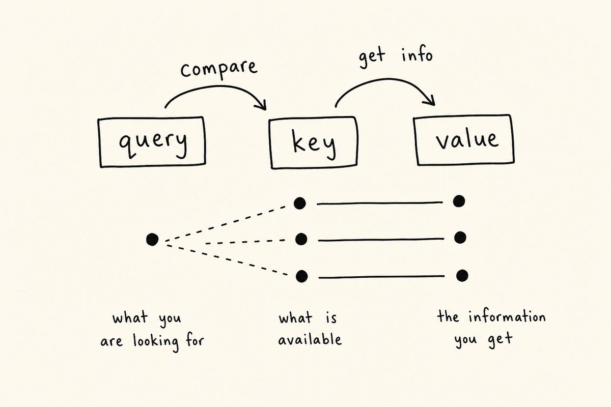
For each token, we create three vectors from its embedding:
- Query (Q): What am I looking for?
- Key (K): What do I contain?
- Value (V): What will I pass if you look at me?
Then for token i, we compare its Query to all Keys (dot product), get attention scores, softmax to get probabilities, and weighted sum of Values.
Example with your prompt "From Prompt to Response Inside an LLM":
For token "Response", Query asks "what modifies me?"
- Key of "From" -> score low 0.05
- Key of "Prompt" -> score high 0.32 because Prompt to Response is a pair
- Key of "to" -> score medium 0.12
- Key of "Inside" -> score medium 0.18
- Key of "LLM" -> score high 0.33 because Response Inside LLM is related
After softmax, weights sum to 1.0, say [0.05, 0.32, 0.12, 0.33, 0.18]. Then output for "Response" = 0.05V_From + 0.32V_Prompt + ...
This new vector now encodes "Response in context of Prompt and LLM" not isolated "Response".
Multi-Head Attention - Why Multiple Heads Matter
Instead of one attention, we run 32 heads in parallel (in Llama 3 8B). Each head learns different relationship type.
Visualization from research:
- Head 3: Tracks subject-verb
- Head 7: Tracks prepositional objects (Prompt -> to -> Response)
- Head 12: Tracks long-range coreference
- Head 21: Attends to next token for local grammar
You combine 32 heads output into one vector. That is why model can handle grammar, facts, and reasoning at same time.
Table: Attention Variants Production Models Use
| Variant | Used In | What It Solves | Tradeoff |
| --- | --- | --- | --- |
| Standard MHA | Original Transformer, GPT-3 | Baseline quality | High KV-cache memory O(n) |
| Multi-Query Attention MQA | Falcon, PaLM | One K/V head shared across Q heads, less memory | Slight quality drop |
| Grouped-Query Attention GQA | Llama 3, Mistral | Groups of Q share K/V, middle ground | Best production compromise |
| FlashAttention-2 | Llama 3 training, vLLM inference | Faster, less HBM to SRAM transfers, same math | Needs implementation support |
| Sliding Window | Mistral 7B | Attend only to last 4096 tokens, linear cost | Loses very long-range |
Production tip: If you host Llama 3, you get GQA by default. GQA cuts KV-cache memory by 4x vs MHA.
Prompt to Visualize Attention:
> "Act as attention visualizer. For sentence 'From Prompt to Response Inside an LLM' explain which tokens token 'Response' would attend to most heavily in head that tracks conceptual pairs. Give weights table and reason."
## Part 4: Step 4 - The Deep Stack - Why Many Layers Matter
One attention layer is not enough. Real model stacks 32 layers (Llama 3 8B) to 96 layers (GPT-4 class).
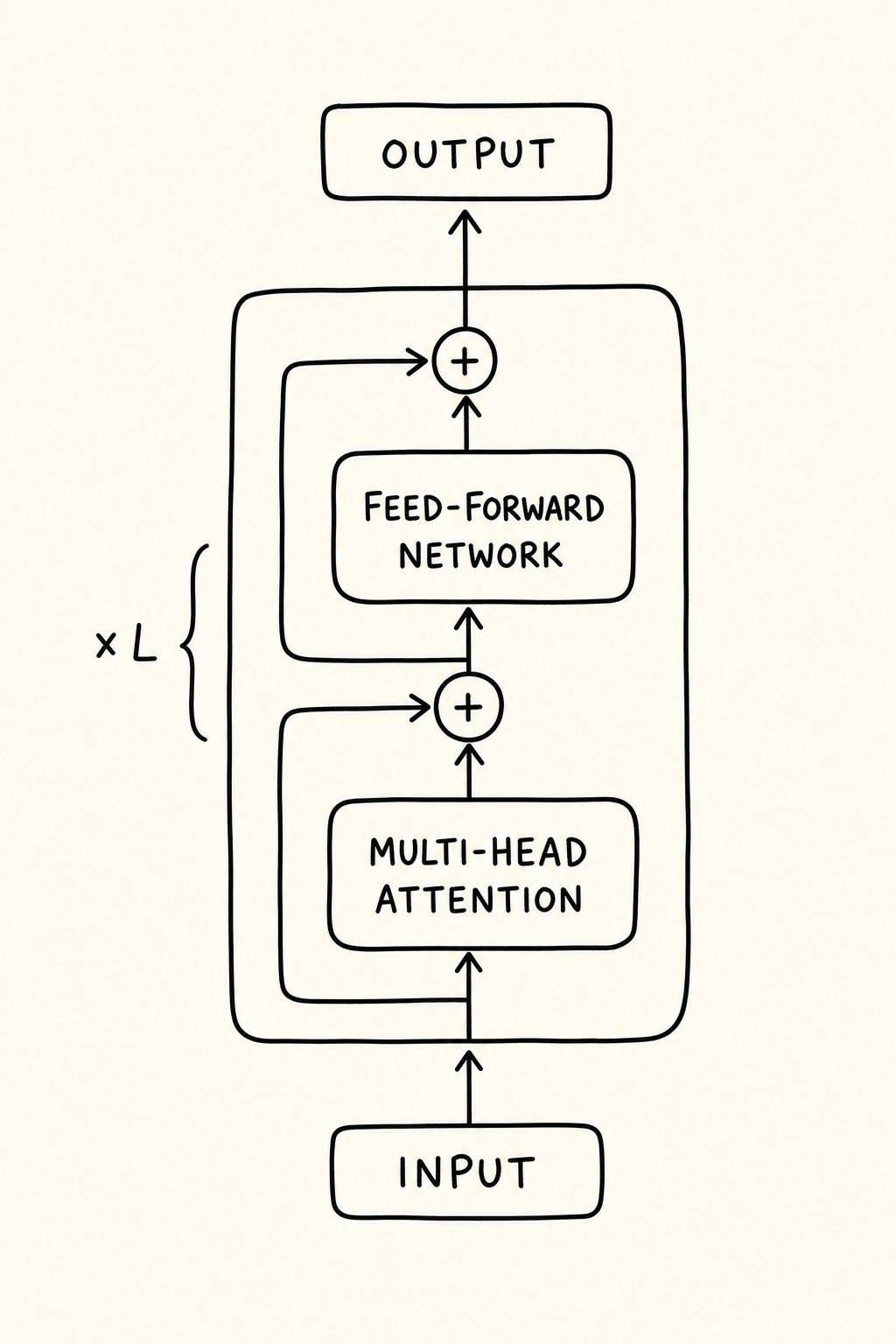
Each layer does:
1. Self-attention
2. Add and LayerNorm (residual connection - keeps previous meaning plus new)
3. Feed-Forward Network (FFN) - two linear layers with SiLU activation that expands to 14336 dim then back to 4096. This is where factual knowledge is stored.
4. Add and LayerNorm again
Mental model:
- Layer 1-8: Learn syntax, grammar, local patterns
- Layer 8-20: Learn semantics, entity relationships
- Layer 20-32: Learn reasoning, task planning, producing final representation for next token
Residual connections are critical. Without them, gradient vanishes and early layer info lost.
Code Example 3: Pseudocode of One Transformer Layer
```
def transformer_layer(x, layer_weights):
# x shape [seq_len, dim]
# 1. Self attention block
residual = x
x = layer_norm(x)
q = x @ W_q # query projection
k = x @ W_k
v = x @ W_v
attn_out = attention(q, k, v) # softmax(QK^T/sqrt(d)) * V
x = residual + attn_out # residual
# 2. FFN block
residual2 = x
x = layer_norm(x)
# FFN is where knowledge lives: up-project then down-project
hidden = silu(x @ W_gate) * (x @ W_up) # SwiGLU variant in Llama 3
ffn_out = hidden @ W_down
x = residual2 + ffn_out
return x
# Stack 32 times
for layer in range(32):
embeddings = transformer_layer(embeddings, weights[layer])
```
After 32 layers, the last token's vector is richest. That vector is used to predict next token.
## Part 5: Step 5 - The Memory Trick - KV-Cache - Why First Token is Slow
If you naively run attention, for each new token you recompute K and V for all previous tokens. For 1000 tokens, that is O(n^2) = 1M operations per layer.
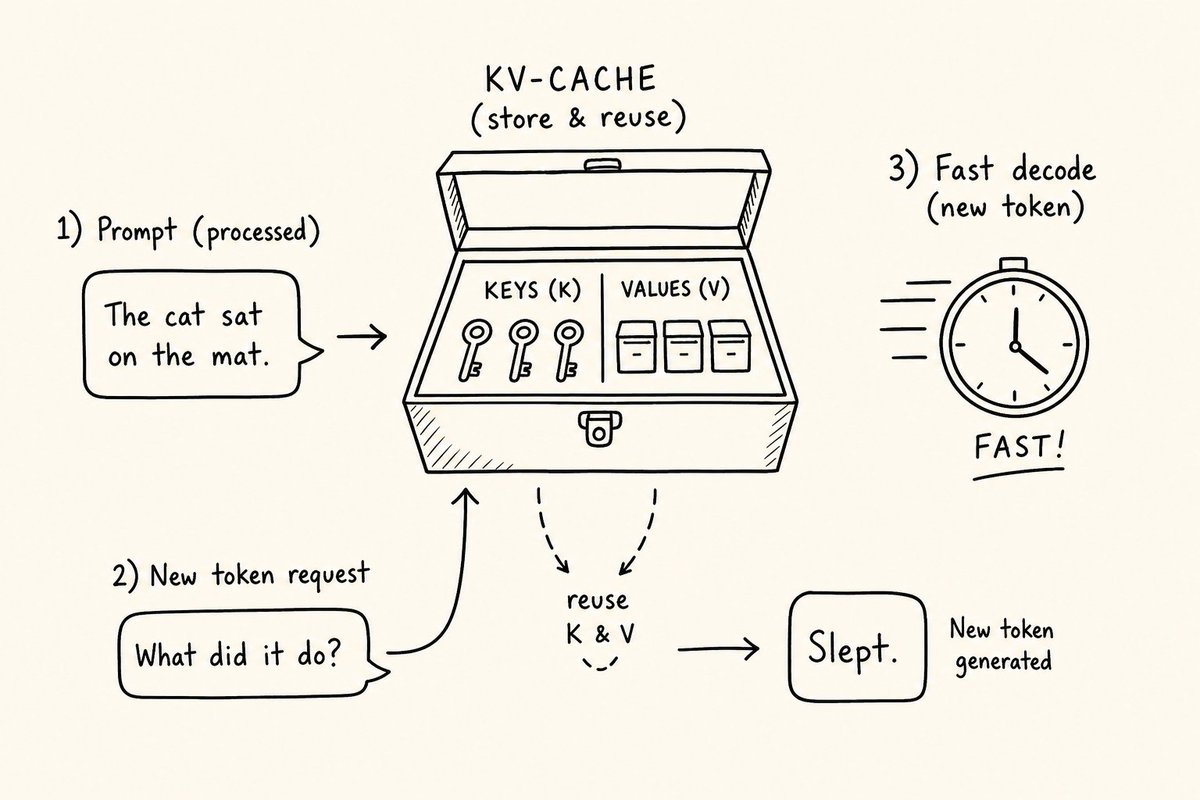
KV-cache stores K and V of previous tokens so you only compute for new token.
- First token (prefill phase): Compute embeddings for full prompt, compute K,V for all prompt tokens, store in cache. This is slow because parallel but heavy.
- Second token onwards (decode phase): Only compute Q,K,V for new token, reuse cached K,V for previous tokens, dot product Q_new with K_all_cached. Fast.
This is why you see latency pattern:
- Time to first token (TTFT): 300ms for 2k prompt
- Inter-token latency (ITL): 20ms per token after
Table: KV-Cache Impact
| Context Length | Without KV-Cache Memory | With KV-Cache Memory per Token | Latency without Cache | Latency with Cache |
| --- | --- | --- | --- | --- |
| 2k tokens | Recalculates all | ~0.5 MB per token (GQA) | High O(n^2) | Fast |
| 32k tokens | Impossible | ~1 MB per token x 32k = 32GB | Timeout | High but possible with paging |
| 128k tokens | Impossible | Needs quantization / offloading | -- | Needs vLLM PagedAttention |
Production performance trick: vLLM and TensorRT-LLM use PagedAttention - they store KV-cache in non-contiguous blocks like OS memory pages, so no fragmentation.
If your LLM is slow on first token but fast after, that is prefill vs decode. Optimize prompt length for TTFT, optimize KV-cache for throughput.
## Part 6: Step 6 - From Vectors to Words - Logits, Softmax, Decoding
After final layer, we have vector for last position, say final_vector dim 4096.
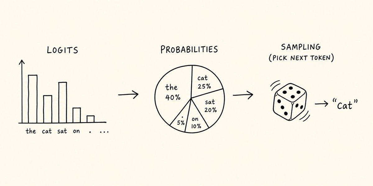
We project it to vocabulary size via unembedding matrix: logits = final_vector @ W_unembed where W_unembed is vocab_size x dim, say 128k x 4096.
Logits are raw unnormalized scores for each possible next token. Example:
```
token " the": logits 12.3
token " a": logits 11.8
token " response": logits 9.1
token " banana": logits -5.2
...
```
Apply softmax to get probabilities:
```
probs = softmax(logits) # sum to 1.0
# " the": 0.42, " a": 0.25, " response": 0.08, ...
```
Now we sample.
Decoding Strategies - Why Same Prompt Gives Different Outputs
Table: Decoding Strategies Comparison
| Strategy | How It Works | Temperature Example | When to Use | Risk |
| --- | --- | --- | --- | --- |
| Greedy | Always pick max probability token | N/A | Deterministic eval, code generation where correctness > creativity | Repetitive, boring |
| Temperature | Divide logits by temp before softmax. Low temp sharpens distribution, high temp flattens | temp 0.2 = focused, 0.8 = creative, 1.2 = wild | Creative writing high temp, factual QA low temp | High temp = hallucination |
| Top-k | Only consider top k tokens | k=50 + temp 0.7 | Old method, simple control | Ignores tail importance |
| Top-p (nucleus) | Consider smallest set where cumulative prob >= p | p=0.9 common | Best general default, dynamic vocab cutoff | Can still cut too much if p low |
| Beam Search | Keep best B beams, expand | beams=4 | Translation, where global coherence matters | Slow, not for chat LLMs |
Code Example 4: Implement Sampling Strategies
```
import torch
import torch.nn.functional as F
def sample_next_token(logits, temperature=0.7, top_p=0.9):
# Temperature scaling
logits = logits / temperature
probs = F.softmax(logits, dim=-1)
# Top-p filtering
sorted_probs, sorted_indices = torch.sort(probs, descending=True)
cumulative_probs = torch.cumsum(sorted_probs, dim=-1)
# Remove tokens with cumulative prob > top_p
sorted_indices_to_remove = cumulative_probs - sorted_probs > top_p
sorted_probs[sorted_indices_to_remove] = 0
sorted_probs = sorted_probs / sorted_probs.sum() # renormalize
# Sample
next_token = torch.multinomial(sorted_probs, num_samples=1)
# Map back to original vocab index
next_token_id = sorted_indices[next_token]
return next_token_id
# Example
# logits from model: shape [vocab_size]
# next_id = sample_next_token(logits, temperature=0.2, top_p=0.95) for factual
# next_id = sample_next_token(logits, temperature=0.9, top_p=0.9) for creative
```
Real LLM inference runs this loop:
```
for step in range(max_new_tokens):
final_vector = model(tokens_so_far)
logits = unembed(final_vector[-1])
next_id = sample(logits, temp, top_p)
tokens_so_far.append(next_id)
if next_id == EOS: break
```
That is why generation is autoregressive - one token at a time, each depends on previous.
## Part 7: Putting It All Together - Walkthrough of Your Prompt
Let us trace "From Prompt to Response Inside an LLM" -> model generating "Here is how..." response.
1. Tokenization: 7 tokens -> IDs [17346, 14508, 284, 24796, 2310, 260, 12382]
2. Embedding: 7 vectors 4096-dim each + RoPE position
3. Layer 1: Each token attends to previous tokens, learns "From ... to ..." structure
4. Layers 2-10: Model recognizes this is meta question about LLM internals, retrieves relevant knowledge from FFN weights where explanations stored
5. Layers 10-30: Planning - decides structure will be intro, steps, conclusion. Last token representation now encodes intent "needs beginner-friendly explanation"
6. Prefill ends: KV-cache holds K,V for 7 prompt tokens
7. Decode step 1: final_vector -> logits -> "Here" highest prob 0.31 at temp 0.7, sampled
8. Decode step 2: Input now 8 tokens (7 prompt + "Here"). Uses KV-cache from 7 + computes Q for "Here", predicts " is"
9. ... repeats 200 times until EOS
Total compute: Prefill heavy on FLOPs, decode heavy on memory bandwidth for KV-cache.
## Part 8: Step 7 - Training to Alignment - Why Model Behaves Like Assistant, Not Just Predictor
Raw pre-trained model predicts internet text. It would continue your prompt with random forum text.
To become assistant, three more stages:
| Stage | Data | Goal | Example |
| --- | --- | --- | --- |
| Pre-training | 15T tokens internet | Learn language and facts | Predict next token on web |
| Supervised Fine-Tuning SFT | 100k instruction + ideal response pairs | Learn to follow instructions | Prompt: Explain X -> Ideal explanation |
| RLHF / DPO | Human preference rankings: Response A better than B | Align to helpful, harmless, honest | Rank responses for safety |
System prompt is then prepended at inference: "You are helpful AI assistant..." - it sits in KV-cache as cached context that steers attention for all future tokens.
Guardrails are extra classifier models that check prompt and response for policy violation before token reaches you.
Hallucination happens because sampling can pick 0.08 probability token "response" over 0.42 "the" when temperature high and top-p allows it, or because FFN stored false knowledge.
## Part 9: Mental Model Checklist - Think Like LLM
Before you prompt next time, run this 5-point check:
- Is my prompt token efficient? Count tokens, remove filler
- Does order help attention? Put important instruction last (recency bias in attention) and also first (system), repeat middle
- Is temperature right? 0.1-0.3 for factual/code, 0.7-0.9 for creative/brainstorm
- Am I using KV-cache well? For same system prompt reuse across calls, cache it (prompt caching in Anthropic/OpenAI can cut 90 percent cost)
- Is expected output short? Long outputs accumulate KV-cache and drift. Ask for structured, bounded answer.
Prompt for Debugging LLM Behavior:
> "Given prompt [X] and model response [Y] that seems off, analyze through lens of tokenization, attention, and decoding: 1) Are any words split into many tokens causing confusion? 2) Which earlier tokens likely got high attention weight causing this? 3) Would lowering temperature or using top-p 0.8 fix it? Give revised prompt."
## Conclusion
From Prompt to Response is not magic. It is engineering:
Tokenize efficient chunks, embed into meaning space, add position, let attention figure out which words matter to which, refine through 32+ layers of FFN where knowledge lives, cache K and V to remember, project to vocabulary probability, sample with temperature and top-p, repeat autoregressively, and steer with SFT and RLHF so it behaves like helpful assistant.
Understand this pipeline and you can debug why your prompt failed, why first token is slow, why same prompt gives different outputs, and how to make it faster and more accurate.
If you can visualize token flow through attention heads and control decoding, you already understand more than 90 percent of LLM users.
## 相关链接
- [Vikas gupta](https://x.com/vicky_grok)
- [@vicky_grok](https://x.com/vicky_grok)
- [12K](https://x.com/vicky_grok/status/2086315908344266782/analytics)
- [https://example.com](https://example.com/)
- [Upgrade to Premium](https://x.com/i/premium_sign_up)
- [12:57 PM · Aug 9, 2026](https://x.com/vicky_grok/status/2086315908344266782)
- [12.1K Views](https://x.com/vicky_grok/status/2086315908344266782/analytics)
---
*导出时间: 2026/8/15 20:56:44*
---
## 中文翻译
# 从提示到响应:LLM 内部的可视化逐步旅程(附代码)
**作者**: Vikas gupta
**日期**: 2026-08-09T04:57:29.000Z
**来源**: [https://x.com/vicky_grok/status/2086315908344266782](https://x.com/vicky_grok/status/2086315908344266782)
---

你输入“像给12岁孩子一样解释Transformer”,然后按下回车。800毫秒后,你得到了五段回复。
在这800毫秒里,你的6个单词变成了词元(tokens),词元变成了12,288维的向量,这些向量经过了96层注意力机制和前馈网络,与一个能记住先前词元的KV缓存(KV-cache)交互,变成了对100,000个可能下一个单词的概率分布,经过温度和top-p采样,最后被去词元化(detokenized)回可读文本。
大多数解释文章止步于“Transformer魔法”。这篇文章将用你可以运行的代码,向你展示每一步。
## 第1部分:步骤1 - 词元化(Tokenization) - 对模型来说,你的文本不是文本
LLM不读取字符。它们读取词元(tokens)。
词元是模型在训练期间学习到的文本块。它可以是一个完整的单词,如“response”,也可以是单词的一部分,如“prompt”,甚至可以是单个字符。
为什么要词元化?为了平衡词汇表大小和序列长度。如果你使用字符,序列会太长。如果你使用完整单词,词汇表会太大,而且无法处理新词。
**30秒理解BPE(字节对编码)如何工作**
字节对编码(Byte Pair Encoding)从字符开始。它反复合并最频繁出现的相邻字符对。
示例:
- 开始:l o w _ l o w e r _ n e w e s t
- 最频繁对:l o
- 合并:lo w _ lo w e r _ n e w e s t
- 下一个频繁对:lo w -> low
- 继续直到达到词汇表大小,比如10万次合并。
结果:常见词“low”变成一个词元。罕见词“lowermost”变成 low + er + most = 3个词元。

**代码示例1:使用tiktoken实时查看词元化**
```
import tiktoken
# gpt-4o 分词器 cl100k_base 是一个很好的参考
enc = tiktoken.get_encoding("cl100k_base")
prompt = "From Prompt to Response Inside an LLM"
tokens = enc.encode(prompt)
decoded = [enc.decode([t]) for t in tokens]
print(f"文本: {prompt}")
print(f"词元ID: {tokens}")
print(f"解码后的词元: {decoded}")
print(f"词元数量: {len(tokens)}")
# 输出近似值:
# 文本: From Prompt to Response Inside an LLM
# 词元ID: [17346, 14508, 284, 24796, 2310, 260, 12382]
# 解码后的词元: ['From', ' Prompt', ' to', ' Response', ' Inside', ' an', ' LLM']
# 词元数量: 7
# 尝试更长的文本
long_prompt = "From Prompt to Response Inside an LLM: A Visual Step-by-Step Journey"
print(enc.encode(long_prompt), len(enc.encode(long_prompt)))
# 大约14个词元
# 为什么这很重要:你按词元付费,上下文窗口是按词元数量计算的,而不是单词数量
```
实用见解:“ an LLM”是2个词元,但“ an LLM.”是3个词元,因为句号合并方式不同。在开头加一个空格可以为许多模型节省词元 - “ Prompt”是一个词元,而字符串开头的“Prompt”可能是不同的ID。
**表格:词元化示例(cl100k_base)**
| 文本 | 词元数 | 原因 |
| --- | --- | --- |
| Hello | 1 | 词汇表中的常见词 |
| Hello world | 2 | 空格+单词合并 |
| HelloWorld | 2-3 | 驼峰式大小写导致拆分 |
| https://example.com | 4-6 | 符号导致拆分 |
| 123456 | 2-3 | 数字按块进行词元化 |
| | 3-6 | 表情符号多词元,成本高 |
规则:如果你构建RAG(检索增强生成),按词元而不是字符分块。使用tiktoken来计数。
**提示模板:**
> “使用cl100k_base计算此提示[你的提示]的词元数,并建议2个更短的版本,保持含义但使用减少20%的词元。解释哪些单词是多词元的。”
## 第2部分:步骤2 - 嵌入和位置编码 - 将ID转化为含义
词元化后,每个词元ID查找一个嵌入向量。把它想象成含义空间中的一个坐标。
如果词汇表是10万,嵌入维度是4096(如Llama 3 8B),嵌入表就是10万 x 4096 = 仅嵌入层就有4亿参数。
token_id 17346 (From) -> [0.021, -0.134, 0.892, ..., 0.011] 4096个数字。
但是,位置1的“From”和位置10的“From”应该被区别对待,因为顺序很重要。自注意力机制没有内置的顺序概念。所以我们需要添加位置编码。
两种常见类型:
- **绝对位置编码**(原始Transformer):基于位置索引将正弦和余弦波添加到嵌入中。位置1得到波A,位置2得到波B。
- **RoPE(旋转位置编码 - 由Llama 3、Mistral、GPT-4使用)**:在复数空间中将嵌入向量旋转与位置成比例的角度。更适合长上下文外推。
嵌入+位置编码后的结果:你有一个向量序列 [x1, x2, x3, ..., x7],每个都是4096维,既知道词元“是什么”,也知道它“在哪里”。
**代码示例2:使用HuggingFace进行嵌入查找**
```
from transformers import AutoTokenizer, AutoModel
import torch
tokenizer = AutoTokenizer.from_pretrained("meta-llama/Meta-Llama-3-8B-Instruct")
model = AutoModel.from_pretrained("meta-llama/Meta-Llama-3-8B-Instruct")
prompt = "From Prompt to Response"
inputs = tokenizer(prompt, return_tensors="pt")
# inputs.input_ids = 词元ID [1, 17346, ...]
# 仅嵌入层
embeddings = model.model.embed_tokens(inputs.input_ids)
print(embeddings.shape) # torch.Size([1, 5, 4096]) = 批次, 序列长度, 维度
# 比较“prompt”和“response”嵌入的余弦相似度
import torch.nn.functional as F
sim = F.cosine_similarity(embeddings[0][1], embeddings[0][3], dim=0)
print(f"在此上下文中 prompt 与 response 的相似度: {sim:.3f}")
```
在上下文中,“prompt”和“response”距离不远,因为它们在指令数据中经常共同出现。嵌入在注意力之后会变得上下文相关,但最初是静态查找。
## 第3部分:步骤3 - 自注意力(Self-Attention) - 你可以建立直觉的核心魔法
这是创造含义的地方。
目标:对于每个词元,找出哪些其他词元对理解它很重要。
句子:“The bank by the river banked money.”(河边的银行存了钱。)
第一个“bank”应该关注“river”,第二个“bank”应该关注“money”和“banked”。同一个词,根据上下文有不同的含义。
**自注意力4步走(不涉及过多数学)**
对于每个词元,我们从其嵌入中创建三个向量:
- **查询(Query,Q)**:我在找什么?
- **键(Key,K)**:我包含什么?
- **值(Value,V)**:如果你看我,我会传递什么?
然后对于词元i,我们将其查询与所有键(点积)进行比较,得到注意力分数,通过softmax得到概率,然后对值进行加权求和。
以你的提示“From Prompt to Response Inside an LLM”为例:
对于词元“Response”,查询会问“什么修饰我?”
- “From”的键 -> 分数低 0.05
- “Prompt”的键 -> 分数高 0.32,因为“Prompt to Response”是一对
- “to”的键 -> 分数中等 0.12
- “Inside”的键 -> 分数中等 0.18
- “LLM”的键 -> 分数高 0.33,因为“Response Inside LLM”相关
经过softmax后,权重总和为1.0,比如 [0.05, 0.32, 0.12, 0.33, 0.18]。那么“Response”的输出 = 0.05V_From + 0.32V_Prompt + ...
这个新向量现在编码了“在Prompt和LLM上下文中的Response”,而不是孤立的“Response”。
**多头注意力 - 为什么多头很重要**
我们不是只运行一个注意力,而是并行运行32个头(在Llama 3 8B中)。每个头学习不同类型的关系。

研究可视化:
- 头3:追踪主谓关系
- 头7:追踪介词宾语(Prompt -> to -> Response)
- 头12:追踪长距离共指关系
- 头21:关注下一个词元以处理局部语法
你将32个头的输出合并成一个向量。这就是为什么模型能同时处理语法、事实和推理。
**表格:生产模型使用的注意力变体**
| 变体 | 使用于 | 解决的问题 | 权衡 |
| --- | --- | --- | --- |
| 标准MHA | 原始Transformer, GPT-3 | 基线质量 | 高KV缓存内存 O(n) |
| 多查询注意力 MQA | Falcon, PaLM | 一个K/V头在所有Q头间共享,内存更少 | 轻微质量下降 |
| 分组查询注意力 GQA | Llama 3, Mistral | Q组共享K/V,折中方案 | 最佳生产妥协 |
| FlashAttention-2 | Llama 3训练, vLLM推理 | 更快,更少HBM到SRAM传输,数学相同 | 需要实现支持 |
| 滑动窗口 | Mistral 7B | 只关注最后4096个词元,线性成本 | 丢失超长距离信息 |
生产提示:如果你托管Llama 3,默认获得GQA。GQA将KV缓存内存比MHA减少4倍。
**可视化注意力的提示:**
> “充当注意力可视化器。对于句子‘From Prompt to Response Inside an LLM’,解释在追踪概念对的注意力头中,词元‘Response’会最关注哪些词元。给出权重表和原因。”
## 第4部分:步骤4 - 深层堆叠 - 为什么需要很多层
一层注意力是不够的。真正的模型堆叠了32层(Llama 3 8B)到96层(GPT-4级别)。

每一层执行:
1. 自注意力
2. 相加和层归一化(残差连接 - 保留先前的含义加上新的)
3. 前馈网络(FFN) - 两个带有SiLU激活的线性层,扩展到14336维,然后回到4096维。这是存储事实知识的地方。
4. 再次相加和层归一化
心智模型:
- 第1-8层:学习语法、句法、局部模式
- 第8-20层:学习语义、实体关系
- 第20-32层:学习推理、任务规划、为下一个词元生成最终表示
残差连接至关重要。没有它们,梯度会消失,早期层的信息会丢失。
**代码示例3:一个Transformer层的伪代码**
```
def transformer_layer(x, layer_weights):
# x 形状 [序列长度, 维度]
# 1. 自注意力块
residual = x
x = layer_norm(x)
q = x @ W_q # 查询投影
k = x @ W_k
v = x @ W_v
attn_out = attention(q, k, v) # softmax(QK^T/sqrt(d)) * V
x = residual + attn_out # 残差
# 2. FFN块
residual2 = x
x = layer_norm(x)
# FFN是知识所在之处:先升维再降维
hidden = silu(x @ W_gate) * (x @ W_up) # Llama 3中的SwiGLU变体
ffn_out = hidden @ W_down
x = residual2 + ffn_out
return x
# 堆叠32次
for layer in range(32):
embeddings = transformer_layer(embeddings, weights[layer])
```
经过32层后,最后一个词元的向量最丰富。该向量用于预测下一个词元。
## 第5部分:步骤5 - 记忆技巧 - KV缓存 - 为什么第一个词元很慢
如果你天真地运行注意力,对于每个新词元,你需要重新计算所有先前词元的K和V。对于1000个词元,每层就是O(n^2) = 100万次操作。

KV缓存存储先前词元的K和V,这样你只需要计算新词元。
- **第一个词元(预填充阶段)**:为完整提示计算嵌入,为所有提示词元计算K、V,存储在缓存中。这很慢,因为是并行的但计算量大。
- **第二个词元及以后(解码阶段)**:只为新词元计算Q、K、V,复用先前词元的缓存K、V,将Q_new与所有K_cached做点积。速度快。
这就是为什么你会看到这样的延迟模式:
- **首词元时间(TTFT)**:2k提示约300ms
- **词元间延迟(ITL)**:之后每个词元约20ms
**表格:KV缓存影响**
| 上下文长度 | 无KV缓存内存 | 有KV缓存每词元内存 | 无缓存延迟 | 有缓存延迟 |
| --- | --- | --- | --- | --- |
| 2k词元 | 重新计算所有 | 每词元约0.5 MB (GQA) | 高 O(n^2) | 快 |
| 32k词元 | 不可能 | 每词元约1 MB x 32k = 32GB | 超时 | 高但可通过分页实现 |
| 128k词元 | 不可能 | 需要量化/卸载 | -- | 需要vLLM PagedAttention |
生产性能技巧:vLLM和TensorRT-LLM使用PagedAttention - 它们将KV缓存存储在非连续块中,就像操作系统内存页面一样,因此没有碎片化。
如果你的LLM第一个词元慢但之后快,那就是预填充与解码的区别。优化提示长度以改善TTFT,优化KV缓存以提高吞吐量。
## 第6部分:步骤6 - 从向量到单词 - Logits、Softmax、解码
在最后一层之后,我们得到最后一个位置的向量,比如final_vector维度为4096。

我们通过去嵌入矩阵将其投影到词汇表大小:logits = final_vector @ W_unembed,其中W_unembed是词汇表大小 x 维度,比如128k x 4096。
Logits是每个可能的下一个词元的原始未归一化分数。示例:
```
词元 " the": logits 12.3
词元 " a": logits 11.8
词元 " response": logits 9.1
词元 " banana": logits -5.2
...
```
应用softmax得到概率:
```
probs = softmax(logits) # 总和为1.0
# " the": 0.42, " a": 0.25, " response": 0.08, ...
```
现在我们进行采样。
**解码策略 - 为什么相同提示会给出不同输出**
**表格:解码策略比较**
| 策略 | 工作原理 | 温度示例 | 何时使用 | 风险 |
| --- | --- | --- | --- | --- |
| 贪婪 | 总是选择最大概率词元 | 不适用 | 确定性评估,正确性>创造性的代码生成 | 重复、无聊 |
| 温度 | softmax前将logits除以温度。低温使分布尖锐,高温使分布平坦 | 温度0.2 = 专注,0.8 = 创意,1.2 = 狂野 | 创意写作用高温,事实问答用低温 | 高温 = 幻觉 |
| Top-k | 只考虑前k个词元 | k=50 + 温度0.7 | 旧方法,简单控制 | 忽略尾部重要性 |
| Top-p (核采样) | 考虑累积概率 >= p的最小集合 | p=0.9常见 | 最佳通用默认值,动态词汇表截断 | 如果p低,可能截断过多 |
| 束搜索 | 保留最佳B个束,扩展 | 束=4 | 翻译,全局连贯性重要 | 慢,不适用于聊天LLM |
**代码示例4:实现采样策略**
```
import torch
import torch.nn.functional as F
def sample_next_token(logits, temperature=0.7, top_p=0.9):
# 温度缩放
logits = logits / temperature
probs = F.softmax(logits, dim=-1)
# Top-p过滤
sorted_probs, sorted_indices = torch.sort(probs, descending=True)
cumulative_probs = torch.cumsum(sorted_probs, dim=-1)
# 移除累积概率 > top_p的词元
sorted_indices_to_remove = cumulative_probs - sorted_probs > top_p
sorted_probs[sorted_indices_to_remove] = 0
sorted_probs = sorted_probs / sorted_probs.sum() # 重新归一化
# 采样
next_token = torch.multinomial(sorted_probs, num_samples=1)
# 映射回原始词汇表索引
next_token_id = sorted_indices[next_token]
return next_token_id
# 示例
# logits 来自模型:形状 [词汇表大小]
# next_id = sample_next_token(logits, temperature=0.2, top_p=0.95) 用于事实性
# next_id = sample_next_token(logits, temperature=0.9, top_p=0.9) 用于创意性
```
真实的LLM推理运行这个循环:
```
for step in range(max_new_tokens):
final_vector = model(tokens_so_far)
logits = unembed(final_vector[-1])
next_id = sample(logits, temp, top_p)
tokens_so_far.append(next_id)
if next_id == EOS: break
```
这就是为什么生成是自回归的 - 一次一个词元,每个词元依赖于之前的词元。
## 第7部分:整合所有内容 - 你的提示的完整走查
让我们追踪“From Prompt to Response Inside an LLM” -> 模型生成“Here is how...”的响应。
1. **词元化**:7个词元 -> ID [17346, 14508, 284, 24796, 2310, 260, 12382]
2. **嵌入**:7个向量,每个4096维 + RoPE位置
3. **第1层**:每个词元关注之前的词元,学习“From ... to ...”结构
4. **第2-10层**:模型识别出这是一个关于LLM内部的元问题,从存储解释的FFN权重中检索相关知识
5. **第10-30层**:规划 - 决定结构将是引言、步骤、结论。最后一个词元的表示现在编码了“需要初学者友好的解释”的意图
6. **预填充结束**:KV缓存持有7个提示词元的K、V
7. **解码步骤1**:final_vector -> logits -> “Here”在温度0.7下概率最高0.31,被采样
8. **解码步骤2**:输入现在是8个词元(7个提示 + “Here”)。使用来自7个的KV缓存 + 为“Here”计算Q,预测“ is”
9. **...重复200次直到EOS**
总计算量:预填充在FLOPs上密集,解码在KV缓存的存储带宽上密集。
## 第8部分:步骤7 - 从训练到对齐 - 为什么模型表现得像助手,而不仅仅是预测器
原始的预训练模型预测互联网文本。它会用随机的论坛文本继续你的提示。
要成为助手,还需要三个阶段:
| 阶段 | 数据 | 目标 | 示例 |
| --- | --- | --- | --- |
| 预训练 | 15万亿词元的互联网数据 | 学习语言和事实 | 在网页上预测下一个词元 |
| 监督微调 SFT | 10万条指令 + 理想响应配对 | 学习遵循指令 | 提示:解释X -> 理想解释 |
| RLHF / DPO | 人类偏好排名:响应A优于响应B | 对齐到有帮助、无害、诚实 | 对响应进行安全排名 |
系统提示在推理时被前置:“你是有帮助的AI助手...” - 它作为缓存的上下文存在于KV缓存中,为所有未来的词元引导注意力。
护栏是额外的分类器模型,在词元到达你之前检查提示和响应是否违反策略。
幻觉发生是因为当温度高且top-p允许时,采样可能选择概率0.08的“response”而不是0.42的“the”,或者因为FFN存储了错误的知识。
## 第9部分:心智模型清单 - 像LLM一样思考
下次你输入提示之前,运行这个5点检查:
- **我的提示词元高效吗?** 计算词元数,移除填充词
- **顺序有助于注意力吗?** 把重要指令放在最后(注意力中的近因偏差)也放在开头(系统),中间重复
- **温度合适吗?** 0.1-0.3用于事实/代码,0.7-0.9用于创意/头脑风暴
- **我是否很好地利用了KV缓存?** 对于跨调用复用的相同系统提示,缓存它(Anthropic/OpenAI中的提示缓存可以削减90%成本)
- **期望输出短吗?** 长输出会累积KV缓存并漂移。要求结构化、有边界的答案。
**调试LLM行为的提示:**
> “给定提示[X]和似乎不对的模型响应[Y],通过词元化、注意力和解码的视角分析:1) 是否有单词被拆分成多个词元导致混淆?2) 哪些早期词元可能获得了高注意力权重导致了这个结果?3) 降低温度或使用top-p 0.8会修复它吗?给出修改后的提示。”
## 结论
从提示到响应不是魔法。它是工程:
高效地词元化块,嵌入到含义空间,添加位置,让注意力找出哪些词对哪些词重要,通过32+层存储知识的FFN进行细化,缓存K和V以记住,投影到词汇表概率,用温度和top-p采样,自回归地重复,并用SFT和RLHF引导,使其表现得像有用的助手。
理解这个流程,你就能调试为什么你的提示失败了,为什么第一个词元很慢,为什么相同的提示给出不同的输出,以及如何让它更快更准确。
如果你能可视化词元在注意力头中的流动并控制解码,你已经比90%以上的LLM用户理解得更多。
## 相关链接
- [Vikas gupta](https://x.com/vicky_grok)
- [@vicky_grok](https://x.com/vicky_grok)
- [12K](https://x.com/vicky_grok/status/2086315908344266782/analytics)
- [https://example.com](https://example.com/)
- [升级到Premium](https://x.com/i/premium_sign_up)
- [2026年8月9日 下午12:57](https://x.com/vicky_grok/status/2086315908344266782)
- [12.1K次查看](https://x.com/vicky_grok/status/2086315908344266782/analytics)
---
*导出时间: 2026/8/15 20:56:44*