LLM 推理原理详解:从 Prefill 到 Decode ✍ Avi Chawla🕐 2026-06-29📦 12.1 KB 🟢 已读 𝕏 文章列表 本文深入解析了大语言模型(LLM)推理的计算流程。文章指出,LLM 推理主要包含 Prefill(处理提示词,计算密集型)和 Decode(逐词生成,显存带宽密集型)两个阶段。作者详细阐述了分词、Embedding、Transformer 层及 KV Cache 的工作原理,并分析了 KV Cache 带来的内存挑战及 vLLM 的优化方案。最后,探讨了 DeepSeek-V4 等新架构通过重新设计注意力机制来从根本上压缩 KV Cache 的创新思路。 LLM推理KV CachePrefillDecodeDeepSeekTransformer性能优化 # How LLM Inference Works, Clearly Explained. **作者**: Avi Chawla **日期**: 2026-06-27T11:14:22.000Z **来源**: [https://x.com/_avichawla/status/2071201619530956863](https://x.com/_avichawla/status/2071201619530956863) --- 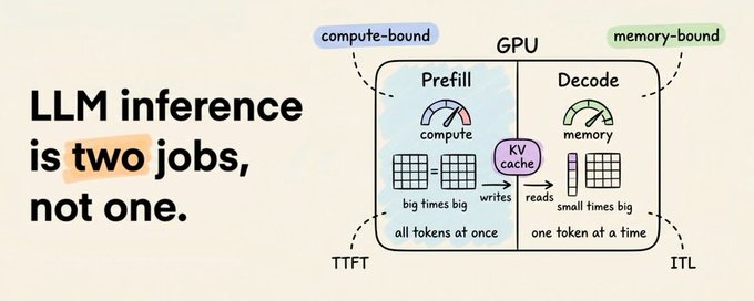 Every generate() call to an LLM runs two distinct computational phases on the same GPU: - prefill (processing the prompt) is compute-bound - while decode (generating tokens one at a time) is memory-bound. Most inference optimizations target one phase or the other, and diagnosing which phase is the bottleneck is the first step in making a deployment faster. In this article, I'll walk through the full pipeline, from tokenized input to streamed output, and look at where the time goes in each phase. # Tokenization and embedding Tokenizers like Byte Pair Encoding (BPE) convert raw text into integer IDs from a vocabulary of roughly 50,000 tokens. ``` prompt = "How does inference work?" ids = tokenizer.encode(prompt) # ids -> [2437, 1374, 32278, 670, 30] ``` Each ID maps to a row in the embedding table, a learned matrix of shape [vocab_size, hidden_dim]. For a model with a hidden dimension of 4,096, each token becomes a 4,096-dimensional vector. ``` # embedding_table has shape [vocab_size, hidden_dim] vectors = embedding_table[ids] # shape: [num_tokens, 4096] ``` 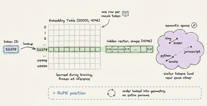 Position information gets injected at this stage. Most modern architectures use Rotary Position Embeddings (RoPE), which encode position by rotating the embedding vectors rather than adding a separate positional vector. # Transformer layers The embedded sequence passes through a stack of transformer layers (typically 32 to 80+, depending on model size). Each layer applies two operations in sequence: 1) Self-attention computes three projections per token (query Q, key K, value V) via learned weight matrices. 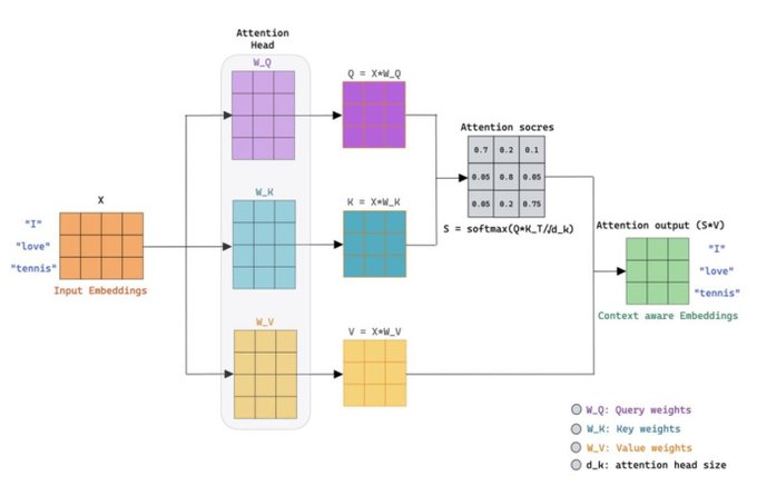 Each token's query is scored against every other token's key, and those scores (after scaling and softmax) determine how much of each token's value gets mixed in. ``` # scores: how much each token attends to every other token Q, K, V = x @ Wq, x @ Wk, x @ Wv scores = (Q @ K.T) / sqrt (d_k) weights = softmax(scaled) # one row per token, sums to 1 attn_output = weights @ V ``` 2) Feed-forward network (FFN) processes each token's vector independently through a two-layer MLP. Attention moves information between positions. The FFN transforms it. After the final layer, the model projects the last token's hidden state back to vocabulary size ([hidden_dim, vocab_size]), applies softmax, and samples from the resulting distribution to produce the first output token. # Prefill: the compute-bound phase Processing the input prompt is the first phase. All tokens are processed in parallel: Q, K, and V are computed for every token simultaneously, and attention runs as a large matrix-matrix multiplication. This is compute-bound work. The GPU's arithmetic throughput is the bottleneck, and utilization is high. The metric that captures this phase is Time to First Token (TTFT), the latency before the first output token appears. During prefill, the model also populates the KV cache: the K and V tensors for every layer get stored in GPU memory for reuse. ``` # Prefill: process the whole prompt in one shot hidden = embed(prompt_tokens) + positions for layer in model.layers: Q, K, V = project(hidden) # for ALL tokens at once hidden = attention(Q, K, V) + hidden hidden = feedforward(hidden) + hidden cache_kv(layer, K, V) # save for later first_token = sample(project_to_vocab(hidden[-1])) ``` # Decode: the memory-bound phase Once the first token is generated, the model switches to generating one token at a time. For each new token, it only computes Q, K, and V for that single token. The K and V from all previous tokens are already in the cache. ``` # Decode: one token per iteration token = first_token steps = 0 while token != STOP and steps < MAX_STEPS: x = embed(token) + position(steps) for layer in model.layers: q, k, v = project(x) K_all, V_all = caches[layer].append(k, v) # cached history + new x = layer.forward(q, K_all, V_all, x) # attention + FFN, residuals token = sample(project_to_vocab(x)) steps += 1 yield token ``` The arithmetic per step is tiny (one query vector against the cached key matrix instead of a full matrix-matrix multiply). But the GPU still loads every weight matrix and the entire cached K/V from memory for that small computation. The bottleneck flips from compute to memory bandwidth. 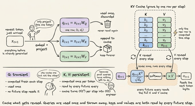 The metric for this phase is Inter-Token Latency (ITL): the time between consecutive output tokens. Low ITL is what makes a model feel responsive. # The KV cache Without caching, generating a 1,000-token response would require recomputing attention over the entire growing sequence at every step, giving quadratic complexity. The KV cache stores each layer's K and V tensors once and appends new entries incrementally. The video below depicts LLM inference speed with vs. without KV caching: 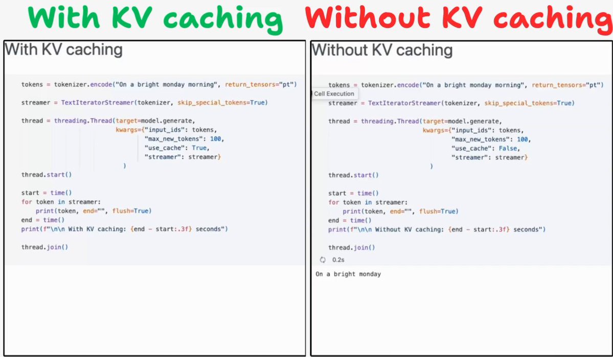 The speedup is roughly 5x or more for long generations. The cost is that the cache grows linearly with sequence length and exists per-layer. For a 13B-parameter model, the cache consumes roughly 1 MB per token. A 4K-token context burns through 4 GB of VRAM on the cache alone. This is why long contexts get expensive. The cache competes directly with batch size for GPU memory, i.e., more cache per request means fewer concurrent requests per GPU. Standard mitigations include quantizing the cache to INT8 or INT4, sliding window attention (dropping tokens outside a fixed window), grouped-query attention (GQA, sharing K/V across attention heads to reduce the number of cached tensors), and PagedAttention (the memory management trick behind vLLM that pages the cache like an OS pages virtual memory, eliminating fragmentation). There's another interesting idea that I talked about around KV cache management below: > **Avi Chawla@_avichawla**: [原文链接](https://x.com/_avichawla/status/2070828078247604480) > > A tricky LLM interview question: > You're serving a reasoning model on vLLM, and it keeps running out of GPU memory on long traces. > So you add KV cache compression and evict 90% of the cached tokens. > VRAM usage stays as is and GPU still runs out of memory. > Why? > (answer below) > > 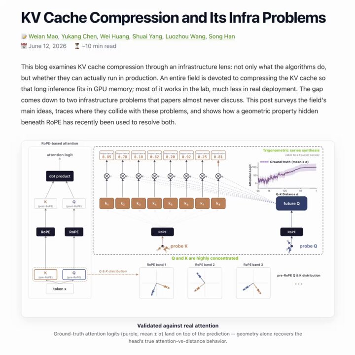 # Redesigning attention around the cache Quantization and paging treat the KV cache as a fixed cost to manage. DeepSeek's V4 series (released April 2025) takes a different approach: redesign attention so the cache is structurally smaller from the start. 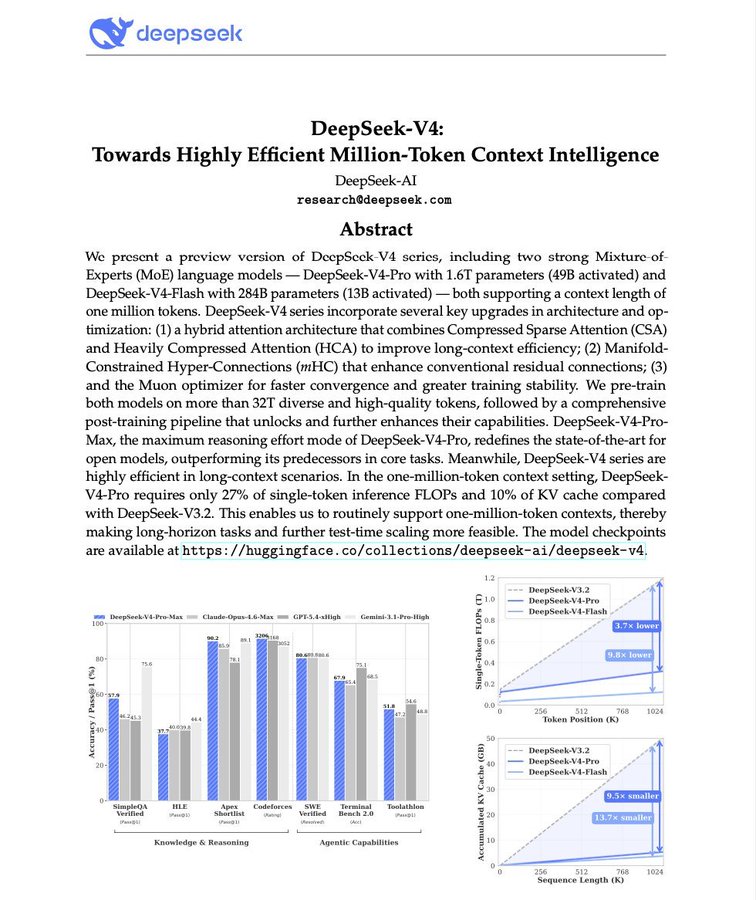 V4 uses a hybrid of two compressed attention mechanisms. Compressed Sparse Attention (CSA) compresses KV entries by 4x using softmax-gated pooling, then applies sparse attention over the compressed tokens. Heavily Compressed Attention (HCA) is more aggressive. It consolidates KV entries across 128 tokens into a single compressed entry and applies dense attention over those representations. At a 1M-token context, V4-Pro requires 27% of the single-token inference FLOPs and 10% of the KV cache compared to DeepSeek-V3.2. In absolute terms, that's 9.62 GiB of KV cache per sequence at 1M context in bf16, compared to an estimated 83.9 GiB for a V3.2-style architecture. With fp4/fp8 quantization on top, the cache shrinks by another 2x. The KV cache has become the constraint that the field is optimizing the model architecture around. # Quantization Training uses FP32 or BF16 for gradient stability. Inference doesn't need that precision. The memory savings from reducing bit width are linear: - 7B parameters at FP32: 28 GB - 7B parameters at FP16/BF16: 14 GB - 7B parameters at INT8: 7 GB - 7B parameters at INT4: 3.5 GB 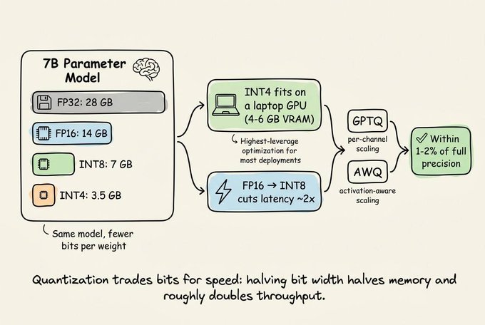 INT4 is why 7B models run on laptop GPUs with 4-6 GB of VRAM. Methods like GPTQ and AWQ use per-channel scaling factors to minimize quality degradation from the lossy compression. Done well, INT4 lands within 1-2 percentage points of the full-precision model on standard benchmarks. Going from FP16 to INT8 often cuts inference latency in half with negligible quality loss, making quantization the single highest-leverage optimization for most deployments. # Serving infrastructure Modern inference servers wrap the prefill-decode loop with several optimizations: 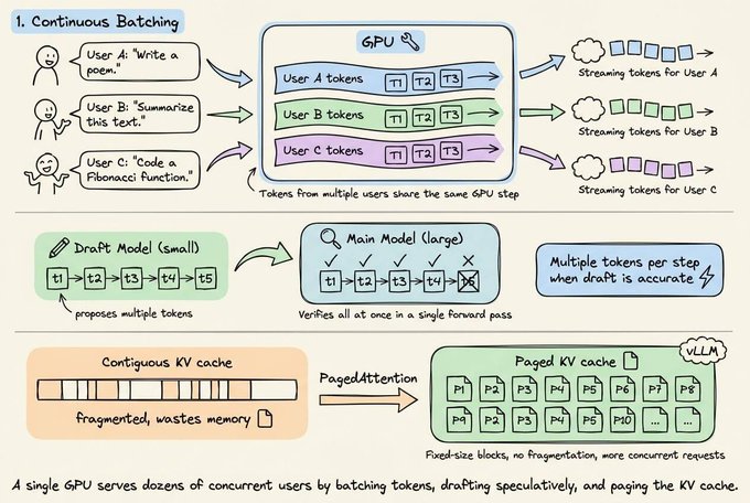 - Continuous batching interleaves tokens from multiple requests on the same GPU step, keeping utilization high even during memory-bound decode phases. - Speculative decoding uses a small draft model to propose multiple tokens, then the large model verifies them in a single forward pass. When the draft model's acceptance rate is high, this effectively converts multiple sequential decode steps into one parallel verification. 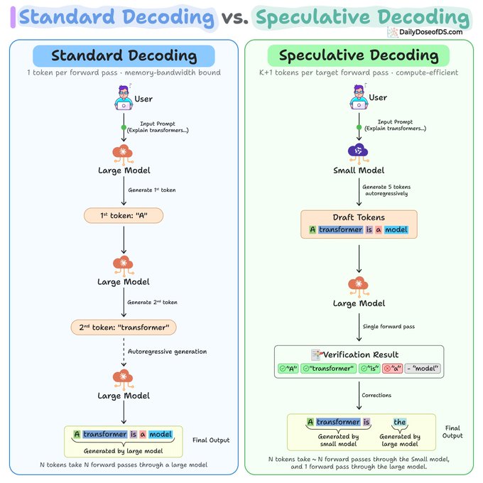 I covered Speculative decoding in detail here: > **Avi Chawla@_avichawla**: [原文链接](https://x.com/_avichawla/status/2054860740541207032) > - PagedAttention (vLLM) manages KV cache memory in fixed-size blocks, eliminating fragmentation and enabling more concurrent requests per GPU. Frameworks like vLLM, TensorRT-LLM, and Text Generation Inference (TGI) combine these techniques. A single GPU can serve dozens of concurrent users because decode leaves most of the arithmetic capacity idle, and continuous batching fills that idle capacity with other requests. # The full inference path 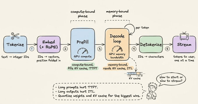 1. Tokenize: Text becomes integer IDs via BPE. 2. Embed: IDs become vectors. RoPE encodes position. 3. Prefill: All input tokens are processed in parallel through every layer. Compute-bound. KV cache populated. First token emitted. 4. Decode loop: One token per step: project Q for the new token, attend over cached K/V, run FFN, sample. Append new K/V to cache. Memory-bound. 5. Detokenize: Token IDs mapped back to text and streamed. # Some practical implications - long prompts are expensive in TTFT (prefill) - long outputs are expensive in ITL (decode) - and they stress different hardware resources. - Context length isn't free because it bloats the KV cache and directly reduces batch capacity. - GPU utilization during decode can drop to 30% even on a fully loaded server, because the bottleneck is memory bandwidth, not arithmetic. - The fix isn't more compute, it's faster memory, a smaller cache, or better batching. When someone tells you their model is slow, the first diagnostic is whether it's slow to start (prefill-bound, optimize TTFT) or slow to stream (decode-bound, optimize ITL). 👉 Over to you: are you running into TTFT or ITL bottlenecks in your deployments, and what's worked for you? That's a wrap! If you enjoyed this tutorial: Find me → @_avichawla Every day, I share tutorials and insights on DS, ML, LLMs, and RAGs. ## 相关链接 - [Avi Chawla](https://x.com/_avichawla) - [@_avichawla](https://x.com/_avichawla) - [28K](https://x.com/_avichawla/status/2071201619530956863/analytics) - [Jun 27](https://x.com/_avichawla/status/2070828078247604480) - [242K](https://x.com/_avichawla/status/2070828078247604480/analytics) - [May 14](https://x.com/_avichawla/status/2054860740541207032) - [39K](https://x.com/_avichawla/status/2054860740541207032/analytics) - [@_avichawla](https://x.com/@_avichawla) - [Upgrade to Premium](https://x.com/i/premium_sign_up) - [7:58 PM · Jun 28, 2026](https://x.com/_avichawla/status/2071201619530956863) - [28.6K Views](https://x.com/_avichawla/status/2071201619530956863/analytics) --- *导出时间: 2026/6/29 12:02:40* --- ## 中文翻译 # LLM 推理的工作原理,清晰讲解。 **作者**: Avi Chawla **日期**: 2026-06-27T11:14:22.000Z **来源**: [https://x.com/_avichawla/status/2071201619530956863](https://x.com/_avichawla/status/2071201619530956863) ---  对 LLM 的每一次 `generate()` 调用,都在同一块 GPU 上运行两个截然不同的计算阶段: - prefill(处理提示词)是计算密集型的 - 而 decode(逐个生成 token)是内存密集型的。 大多数推理优化都针对这两个阶段之一,而诊断哪个阶段是瓶颈是加速部署的第一步。 在这篇文章中,我将梳理从分词输入到流式输出的完整流程,并看看每个阶段的时间都花在哪里了。 # 分词与嵌入 像字节对编码(BPE)这样的分词器会将原始文本转换为大约 5 万个词表大小对应的整数 ID。 ``` prompt = "How does inference work?" ids = tokenizer.encode(prompt) # ids -> [2437, 1374, 32278, 670, 30] ``` 每个 ID 都映射到嵌入表中的一行,这是一个形状为 [vocab_size, hidden_dim] 的学习矩阵。对于一个隐藏层维度为 4,096 的模型,每个 token 都会变成一个 4,096 维的向量。 ``` # embedding_table 的形状为 [vocab_size, hidden_dim] vectors = embedding_table[ids] # shape: [num_tokens, 4096] ```  位置信息在此阶段被注入。 大多数现代架构使用旋转位置编码,它通过旋转嵌入向量来编码位置,而不是添加单独的位置向量。 # Transformer 层 嵌入后的序列会通过一堆 Transformer 层(通常是 32 到 80 多层,取决于模型大小)。 每一层按顺序应用两个操作: 1) **自注意力** 通过学习的权重矩阵为每个 token 计算三个投影(Query Q, Key K, Value V)。  每个 token 的 Query 都会与其他所有 token 的 Key 进行打分,这些分数(经过缩放和 softmax 后)决定了每个 token 的 Value 有多少被混合进来。 ``` # scores: 每个 token 对其他所有 token 的关注度 Q, K, V = x @ Wq, x @ Wk, x @ Wv scores = (Q @ K.T) / sqrt (d_k) weights = softmax(scaled) # 每个 token 一行,总和为 1 attn_output = weights @ V ``` 2) **前馈网络(FFN)** 通过一个两层 MLP 独立处理每个 token 的向量。注意力负责在位置之间传递信息。FFN 负责对其进行转换。 在最后一层之后,模型会将最后一个 token 的隐藏状态投影回词表大小([hidden_dim, vocab_size]),应用 softmax,并从结果分布中进行采样,以产生第一个输出 token。 # Prefill:计算密集型阶段 处理输入提示词是第一阶段。所有 token 都被并行处理:同时计算每个 token 的 Q、K 和 V,并且注意力运算作为一个大型矩阵-矩阵乘法运行。 这是计算密集型工作。GPU 的算力吞吐量是瓶颈,利用率很高。衡量这一阶段的指标是首字延迟,即第一个输出 token 出现之前的延迟。 在 Prefill 阶段,模型还会填充 KV 缓存:每一层的 K 和 V 张量会被存储在 GPU 内存中供后续重用。 ``` # Prefill: 一次性处理整个提示词 hidden = embed(prompt_tokens) + positions for layer in model.layers: Q, K, V = project(hidden) # 一次性处理所有 token hidden = attention(Q, K, V) + hidden hidden = feedforward(hidden) + hidden cache_kv(layer, K, V) # 留作后用 first_token = sample(project_to_vocab(hidden[-1])) ``` # Decode:内存密集型阶段 一旦生成了第一个 token,模型就会切换到一次生成一个 token 的模式。对于每一个新 token,它只计算该单个 token 的 Q、K 和 V。所有之前 token 的 K 和 V 已经在缓存中了。 ``` # Decode: 每次迭代一个 token token = first_token steps = 0 while token != STOP and steps < MAX_STEPS: x = embed(token) + position(steps) for layer in model.layers: q, k, v = project(x) K_all, V_all = caches[layer].append(k, v) # 缓存的历史记录 + 新的 x = layer.forward(q, K_all, V_all, x) # attention + FFN, 残差 token = sample(project_to_vocab(x)) steps += 1 yield token ``` 每一步的计算量非常小(是一个 query 向量与缓存 key 矩阵的计算,而不是完整的矩阵-矩阵乘法)。但是 GPU 仍然需要为这少量的计算从内存中加载每一个权重矩阵和整个缓存的 K/V。瓶颈从计算翻转为内存带宽。  衡量这一阶段的指标是 Token 间延迟(ITL):连续输出 token 之间的时间。低 ITL 是让模型感觉响应迅速的关键。 # KV 缓存 如果没有缓存,生成一个 1,000 token 的响应就需要在每一步重新计算整个不断增长的序列的注意力,导致二次复杂度。 KV 缓存将每一层的 K 和 V 张量存储一次,并增量追加新条目。 下面的视频展示了有无 KV 缓存时的 LLM 推理速度对比:  对于长文本生成,加速比大约在 5 倍以上。 代价是缓存的大小随序列长度线性增长,并且每一层都有一份。对于一个 13B 参数的模型,缓存大约占用每个 token 1 MB。一个 4K token 的上下文仅缓存就会消耗掉 4 GB 的显存。 这就是为什么长上下文代价高昂。缓存与批处理大小直接争夺 GPU 内存,即每个请求的缓存越多,意味着每块 GPU 上能处理的并发请求就越少。 常见的缓解措施包括将缓存量化为 INT8 或 INT4、滑动窗口注意力(丢弃固定窗口之外的 token)、分组查询注意力(GQA,在注意力头之间共享 K/V 以减少缓存张量的数量)以及 PagedAttention(vLLM 背后的内存管理技巧,像操作系统分页虚拟内存一样对缓存进行分页,消除碎片)。 还有一个关于 KV 缓存管理的有趣观点,我在下面谈到过: > **Avi Chawla@_avichawla**: [原文链接](https://x.com/_avichawla/status/2070828078247604480) > > 一个棘手的 LLM 面试题: > 你在 vLLM 上部署一个推理模型,但在长轨迹上总是耗尽 GPU 内存。 > 所以你添加了 KV 缓存压缩并驱逐了 90% 的缓存 token。 > 显存(VRAM)使用量保持不变,GPU 依然内存不足。 > 为什么? > (答案在下方) > >  # 围绕缓存重新设计注意力机制 量化和分页将 KV 缓存视为需要管理的固定成本。DeepSeek 的 V4 系列(2025 年 4 月发布)采用了不同的方法:重新设计注意力机制,使得缓存从结构上从一开始就更小。  V4 使用了两种压缩注意力机制的混合体。 压缩稀疏注意力(CSA)通过 softmax 门控池化将 KV 条目压缩 4 倍,然后对压缩后的 token 应用稀疏注意力。 重度压缩注意力(HCA)则更为激进。它将 128 个 token 的 KV 条目合并为一个单一的压缩条目,并对这些表示应用密集注意力。 在 100 万 token 的上下文中,V4-Pro 仅需相当于 DeepSeek-V3.2 单 token 推理 27% 的 FLOPs 和 10% 的 KV 缓存。 绝对值上,在 bf16 精度下,100 万上下文时每个序列的 KV 缓存为 9.62 GiB,而 V3.2 架构估计为 83.9 GiB。如果在此基础上加上 fp4/fp8 量化,缓存还会再缩小 2 倍。 KV 缓存已成为该领域优化模型架构时的约束条件。 # 量化 训练使用 FP32 或 BF16 以保持梯度稳定。推理不需要那么高的精度。降低位宽带来的内存节省是线性的: - FP32 的 7B 参数:28 GB - FP16/BF16 的 7B 参数:14 GB - INT8 的 7B 参数:7 GB - INT4 的 7B 参数:3.5 GB  正是因为 INT4,7B 模型才能在显存只有 4-6 GB 的笔记本电脑 GPU 上运行。像 GPTQ 和 AWQ 这样的方法使用逐通道缩放因子,将有损压缩带来的质量降至最低。 如果做得好,在标准基准测试中,INT4 的表现与全精度模型相比仅相差 1-2 个百分点。 从 FP16 转到 INT8 通常能在质量损失极小的情况下将推理延迟减半,这使得量化成为大多数部署中杠杆率最高的单一优化手段。 # 服务基础设施 现代推理服务器在 prefill-decode 循环外包裹了多项优化:  - **连续批处理** 在同一个 GPU 步骤中穿插处理来自多个请求的 token,即使在内存密集型的 decode 阶段也能保持高利用率。 - **投机解码** 使用一个小型草稿模型来提出多个 token,然后由大模型在一次前向传播中验证它们。当草稿模型的接受率很高时,这有效地将多个连续的 decode 步骤转换为一个并行验证步骤。  我曾在这里详细介绍过投机解码: > **Avi Chawla@_avichawla**: [原文链接](https://x.com/_avichawla/status/2054860740541207032) > - **PagedAttention** (vLLM) 以固定大小的块管理 KV 缓存内存,消除了碎片,并支持每个 GPU 处理更多并发请求。 像 vLLM、TensorRT-LLM 和 Text Generation Inference (TGI) 这样的框架结合了这些技术。单块 GPU 可以服务数十个并发用户,因为 decode 阶段会让大部分算力闲置,而连续批处理正好用其他请求填补了这些闲置能力。 # 完整的推理路径  1. **分词**:文本通过 BPE 变成整数 ID。 2. **嵌入**:ID 变成向量。RoPE 编码位置。 3. **Prefill**:所有输入 token 通过每一层被并行处理。计算密集型。KV 缓存被填充。输出第一个 token。 4. **Decode 循环**:每步一个 token:为新 token 投影 Q,对缓存的 K/V 计算注意力,运行 FFN,采样。将新的 K/V 追加到缓存。内存密集型。 5. **反分词**:Token ID 映射回文本并流式输出。 # 一些实际启示 - 长提示词在 TTFT(prefill)上代价高昂 - 长输出在 ITL(decode)上代价高昂 - 它们会给不同的硬件资源带来压力。 - 上下文长度不是免费的,因为它会膨胀 KV 缓存并直接降低批处理能力。 - 即使在满载的服务器上,decode 阶段的 GPU 利用率也可能降至 30%,因为瓶颈在于内存带宽,而非算力。 - 解决之道不是更多的计算,而是更快的内存、更小的缓存或更好的批处理。 当有人告诉你他们的模型很慢时,第一步诊断就是判断它是启动慢(prefill-bound,需优化 TTFT)还是流式输出慢(decode-bound,需优化 ITL)。 👉 轮到你了:在你的部署中遇到的是 TTFT 还是 ITL 瓶颈,什么方法对你有效? 总结完毕! 如果你喜欢这个教程: Find me → @_avichawla 每天,我都会分享关于 DS, ML, LLMs 和 RAGs 的教程和见解。
L LLM 优化面试笔记:训练与推理核心技术 这是一份针对 AI 实验室面试准备的笔记,涵盖了高效训练和部署大语言模型(LLM)的核心优化策略。内容主要分为三部分:内存优化(如 Flash Attention、MQA/GQA、激活检查点)、计算优化(序列打包、高效变体 Transformer)以及推理优化(KV 缓存、投机解码、量化技术)。文章旨在总结在大规模模型开发中应对算力和内存瓶颈的关键技术。 技术 › LLM ✍ Gauri Gupta🕐 2026-05-06 LLM优化推理训练Flash AttentionKV Cache量化面试Transformer性能优化
L LLM 原理与实践指南 (2026 版) 这是一份关于大语言模型(LLM)的实践指南。文章从基础循环机制出发,详细解释了文本如何转化为 Token,以及 Transformer、注意力机制、KV Cache 和 RoPE 等核心概念的工作原理。作者强调理解模型内部的推理机制(如 Prefill 和 Decode 阶段)对于硬件选型、显存估算和本地部署的重要性。文章涵盖了 Token 化、上下文窗口、量化、模型服务及本地 AI 硬件数学计算等关键主题,旨在为深入理解 LLM 提供直观的基础。 技术 › LLM ✍ Ahmad🕐 2026-05-23 LLMTransformer本地部署Tokenization推理Attention硬件教程KV Cache
大 大语言模型训练与服务背后的数学原理 本文基于 Reiner Pope 的播客内容,深入剖析了大模型在集群中的运行机制。文章通过 Roofline 分析和 KV Cache 等核心概念,解释了推理延迟、Batch Size、API 定价策略及 MoE 架构背后的物理与经济逻辑,揭示了硬件限制如何塑造 AI 进展。 技术 › LLM ✍ Saito🕐 2026-05-01 LLM推理架构设计数学原理MoEAPI定价性能优化Transformer
F From GPT2 to Kimi3, Explained 文章回顾了从 GPT-2 (2019) 到 KimiK3 (2026) 的大语言模型架构演进,重点对比了参数规模从 1.24 亿到 2.8 万亿的巨大跨越。深入解析了 GPT-2 的 Transformer 解码器结构、KV 缓存机制,并探讨了线性注意力机制在降低计算复杂度方面的原理与权衡。 技术 › LLM ✍ ali🕐 2026-07-28 LLMTransformerKimiK3GPT-2AttentionKV Cache架构演进线性注意力
下 下一代 LLM 推理网络:ZCube 如何缓解网络瓶颈 文章探讨了随着长上下文推理和 Prefill-Decode 解耦成为主流,网络如何成为 LLM 推理集群吞吐量和延迟的关键瓶颈。Z.ai、Harnets.AI 和清华大学联合开发了 ZCube 网络架构,通过扁平化拓扑和混合轨道设计,有效解决了传统 ROFT 架构下的流量负载不均衡问题。生产环境基准测试显示,ZCube 仅通过架构优化便实现了交换机成本降低 33%、吞吐量提升 15% 以及 TTFT 延迟降低 40.6% 的显著收益。 技术 › DevOps ✍ Z.ai🕐 2026-05-21 LLM推理网络架构ZCube性能优化Prefill-Decode负载均衡ROFT基础设施清华大学
D DeepSeek新论文解读:用“手指着图片思考”的多模态推理框架 DeepSeek发布新论文,提出一种名为“视觉原语”的多模态推理框架。不同于业界卷分辨率的趋势,该模型通过在思维链中嵌入边界框和坐标点,模拟人类用手指着图片思考的过程,有效解决了语言在空间指代上的局限。DeepSeek-ViT配合LLM将视觉Token压缩至竞品的十分之一,但在空间推理、计数和迷宫导航等任务上性能超越GPT-5.4等顶尖模型。 技术 › LLM ✍ 向阳乔木🕐 2026-05-01 DeepSeek多模态视觉推理论文解读Transformer人工智能计算机视觉LLM
L LLM 中的 Prompt Caching 技术详解:以 Claude 为例的高效缓存策略 本文深入探讨了 LLM 中的 Prompt Caching 技术,解释了其背后的 KV Cache 机制及静态/动态上下文分离原理。文章通过 Claude Code 的案例分析,展示了如何通过保持 92% 的缓存命中率来将计算成本降低 81%,并总结了哈希敏感性和工程化落地的关键约束。 技术 › LLM ✍ Avi Chawla🕐 2026-04-20 Prompt CachingLLMAgentClaudeKV Cache成本优化系统架构Transformer
L LLM 中的 KV 缓存机制详解 文章深入解释了大型语言模型(LLM)中的 KV 缓存技术。作者指出,LLM 生成文本时首个令牌较慢而后续令牌迅速的现象,归功于 KV 缓存的工程优化。该技术通过存储已计算键值向量,避免在自回归生成过程中的冗余计算,以 GPU 内存为代价换取显著的计算加速。文中详细解析了注意力机制的冗余问题、KV 缓存的工作原理、首令牌延迟(TTFT)的产生原因,以及内存与计算资源之间的权衡取舍。 技术 › LLM ✍ Avi Chawla🕐 2026-03-22 KV缓存注意力机制Transformer模型推理LLM性能优化GPU内存预填充TTC大模型
M Math Behind Large Language Model 本文介绍了大语言模型背后的数学原理,涵盖Attention机制、缩放因子、反向传播、梯度下降、交叉熵损失、RoPE位置编码和RMSNorm归一化等核心概念。 技术 › LLM ✍ Amit Shekhar🕐 2026-07-30 LLM数学原理AttentionTransformer机器学习深度学习梯度下降反向传播RoPERMSNorm
K Kimi K3 memory savings vs Jevon's paradox 本文深入分析了Kimi K3通过Kimi Delta Attention (KDA)技术实现的内存节省突破,对比了传统MLA和DeepSeek的架构,讨论了其在长上下文场景中的优势及对行业的影响。 技术 › LLM ✍ GDP🕐 2026-07-30 Kimi K3KDA内存节省长上下文DeepSeekMLA混合线性注意力KV cache
C CAG:缓存增强生成,RAG的替代方案 文章介绍了缓存增强生成(CAG)作为一种替代经典RAG流水线的新方案。CAG通过将全部知识预加载到模型上下文并缓存KV Cache,显著提升响应速度,解决检索延迟和召回缺失问题。适用于中短篇幅静态文档,但对大规模或频繁变动数据仍需传统RAG或混合架构。 技术 › LLM ✍ Amto🕐 2026-07-29 CAGRAG缓存增强生成LLM私有知识向量化KV Cache开源
P PagedAttention & RadixAttention 本文深入探讨了 PagedAttention 和 RadixAttention 两种技术。PagedAttention 通过类似操作系统的分页机制管理 GPU 内存,解决 KV Cache 的内部和外部碎片问题,显著提升并发处理能力。RadixAttention 则利用基数树索引缓存的前缀状态,实现跨请求的计算和内存复用,进一步优化推理性能。 技术 › LLM ✍ prasanna🕐 2026-07-28 vLLMSGLangPagedAttentionRadixAttentionKV Cache内存管理推理优化LLM