# How robot arms are controlled
**作者**: Jacob H. Rothschild
**日期**: 2026-09-17T17:10:26.000Z
**来源**: [https://x.com/ja_rothschild/status/2100633491432239411](https://x.com/ja_rothschild/status/2100633491432239411)
---
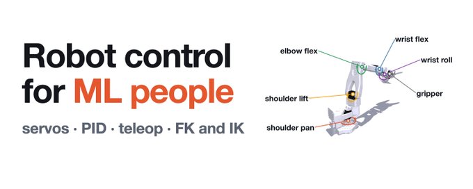
If you're an ML practitioner entering robot learning, directly controlling hardware may seem daunting. My hope is that this article can help you cross that hurdle.
I'll cover how an SO-100 robot arm is composed, how we record data, how it chases targets, how an ML policy can drive it, and the different representations we can use. And I'll explain why, counterintuitively, the arm can reach exactly 0% of the gripper poses (position + orientation) within arm's length.
Note that everything in this article also applies to the newer SO-101, and most of it to any robot arm.
This is the first of the explainers I promised in [Speedrunning robot learning](https://x.com/ja_rothschild/status/2099482366817468515). I'll post the others over the coming week or two.
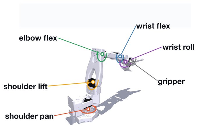
The joints of an SO-100 follower arm.
## Decomposing the arm
The robot I've been studying is the SO-100 arm. It's composed of six links with five joints between them, together determining the gripper's "pose" (its position + orientation). The gripper itself can open and close, thus is an extra joint and link.
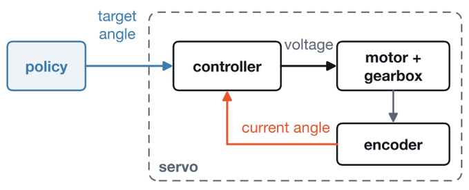
Each joint contains a servo, consisting of a motor, a gearbox, an encoder, and a controller. The controller receives a target angle for its joint and reads the current angle off the encoder. Many times per second it determines the torque to apply and sends the corresponding voltage (a function of torque, gear and speed) to the motor. To control the arm, we thus tell it a few dozen times per second (30 Hz in LeRobot) the target angle of every joint. This is called (joint) position control, and although it isn't the only way to control a servo, it's what the SO-100 uses, thus what we'll cover here.
## Collecting data
Sending target angles is also how demonstrations get recorded. The SO-100 setup consists of a leader arm and a follower arm. The leader is built so that a human can move it by hand against little force. The leader's joint angles are read from its servos and sent to the follower as target angles. By also writing to disk the time series of the leader's joint angles, the follower's joint angles, and the frames of any attached cameras, we get a "teleoperation" dataset of input-output pairs (the leader's angles are the output, the rest is the input).
<video controls preload="metadata" poster="/doc/6820/image/img_493a387f266d.jpg" src="/videos/0725.mp4"></video>
The follower copies the leader's joint angles. Curve colors match the joint labels above: green elbow flex, blue wrist flex, gray gripper, purple wrist roll, red shoulder pan, yellow shoulder lift. Thick pale: leader. Thin: follower.
## Chasing target angles
SO-100 servos use PID controllers. A PID controller is modeled as a spring pulling the joint towards the target angle ("P" for proportional), a damper meant to stop it from overshooting that target ("D" for derivative), and an integral term ("I"). That last term measures systemic bias over time and adds whatever extra torque is necessary to eliminate it, thus canceling external forces that would otherwise move the equilibrium off of the target (e.g. gravity counteracting the spring force). The SO-100 arms set the I term to zero, thus don't correct systemic bias.
Balancing the P and D terms isn't trivial. Underdamp your spring, and you overshoot your target. Overdamp it, and movements become slow. Critical damping is the minimal damping that doesn't overshoot, and for our spring it's reached when the damping gain D (the torque applied per unit of angular velocity) equals 2·√(P·J), where J is the moment of inertia of everything the joint has to swing around. That inertia isn't a constant, since it depends on the pose: the further the rest of the arm sticks out past the joint, the larger J is (for the shoulder lift joint, more than 10x between folded and stretched out, though the motor's own rotor adds a large constant on top that shrinks that ratio a lot). The controller's D, however, is fixed, so the joint can only be critically damped at one value of J. Stretch the arm out further than that and the joint underdamps and overshoots. Fold it in further and it overdamps and crawls.
<video controls preload="metadata" poster="/doc/6820/image/img_0130accfb664.jpg" src="/videos/0726.mp4"></video>
Same joint and spring, three damper strengths. Black circle: target gripper position. Dashed line: target angle. Arrows and bottom curves: the spring and damper torques.
Moreover, a cheap robot arm has quite weak motors, so the torque it can produce is limited. If the target angle changes too drastically or quickly, the sum of the spring and damping torques gets clipped at the motor's max torque, hence becomes a non-linear function of its inputs, and critical damping and a lot of other nice properties of the system fall away.
<video controls preload="metadata" poster="/doc/6820/image/img_fef2a05b9643.jpg" src="/videos/0727.mp4"></video>
A big jump in target angle makes the joint overshoot. Only the 140° step gets too fast to brake in time. Black circle: target gripper position. Dashed line: target angle. Bottom bar: red while the motor is at the MuJoCo model's 3.5 N·m torque limit (first to accelerate the joint, then to decelerate it), gray otherwise.
## Representing state
Now the full arm again. Five joints, each with a legal range, gives us a 5-dimensional "joint space": a cuboid living in R^5, where coordinate i describes the angle of joint i (the gripper adds a sixth coordinate, which I'll leave out here since it doesn't move the arm). What we're often interested in instead is task space: the 6-dimensional space representing the position (x, y, z) and orientation (roll, pitch, yaw) of the gripper. Note that not all points in joint space are physically legal, since over 10% of them would cause links to collide.
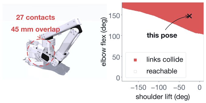
Forward kinematics (FK) is the task of transforming from joint space to task space. It's as simple as starting at the base and running a sequence of rigid transforms (rotation + offset), each determined by the angle of a joint and the geometry of the link right after it. Simulators such as MuJoCo run FK at every physics step (500 Hz by default) to calculate where in space every part of the robot arm is and apply the corresponding physics.
Inverse kinematics (IK) is the inverse of FK: given a point in task space, find a point in joint space that FK would map to it. While FK is unproblematic, IK can be annoying, for three reasons.
First, FK is in general a non-injective function: every point in joint space corresponds to a single point in task space, but multiple points in joint space can correspond to the same point in task space.
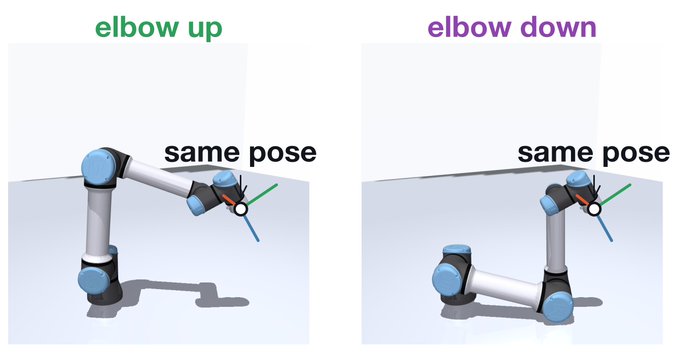
Different joint angles, same gripper pose.
Thus, if a robot policy outputs sequences of target coordinates, we'll have to be careful about which IK solution we choose for each, so that we're not jumping between wildly different joint angles.
<video controls preload="metadata" poster="/doc/6820/image/img_289f32cf3fb8.jpg" src="/videos/0728.mp4"></video>
Same gripper circle on a UR5e, two ways to pick the IK solution. Left: IK solved from scratch at each step. Right: IK started from the previous step's solution.
Second, FK is non-surjective: most points in task space have no FK preimage (a point that FK would map to it), e.g. due to being too far away or requiring joint angles outside the legal range. This is especially acute for the SO-100: FK is smooth and its domain (joint space) lives in R^5, while its codomain (task space) is 6-dimensional, so its image is a lower-dimensional subset of its codomain, hence has Lebesgue measure 0. Put simply, if you (uniformly) randomly draw a target orientation and a target position within arm's length, the probability an SO-100 arm can reach that pose (exactly) is 0%.
Third, FK has singularities (configurations where the Jacobian, the derivative of FK, loses rank), e.g. when the arm is fully extended. Approach or leave a singularity head-on at constant speed (e.g. extend the arm fully while keeping the gripper's speed constant), and the required angular velocities (and torques) go to infinity. The reason is that the reach is maximal at full extension, thus stationary in the elbow angle, so the last ε of reach costs an elbow angle of about √ε, and the slope of √ε at zero is infinite. Our motors, however, bound their angular velocities (and torques), and as a result the controllers fall behind schedule.
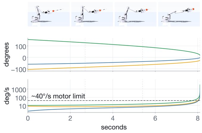
Joint speeds shoot up near full extension, even though the gripper moves at constant speed. Green: elbow flex. Blue: wrist flex. Yellow: shoulder lift. Dashed vertical lines: the snapshot times (first is at t=0).
## Choosing our space
Since our controllers read target angles, a policy that outputs points in task space must first have IK run on an output before the corresponding point in joint space can be sent to the servos. If the training set of the policy spans different robot arms, such as is the case for OpenVLA, it can be easier to learn task space deltas than joint angles, since every arm has a gripper pose, whereas the joints differ from arm to arm. If the policy is instead trained on a single arm (or through zero-padding of missing DoF), we can teach it to directly output joint angles, which is the form the demonstrations come in anyway, and thus sidestep the whole need for IK. ACT and π0 are examples of policies that directly output joint angles. Whether those are absolute angles or deltas from the current pose is a separate choice, and policies exist on both sides. Deltas look the same wherever the arm currently is, which makes them easy to normalize. ACT outputs absolute target angles (and reports that deltas worked worse for it), while π0's official implementation trains on deltas.
So on a single arm, the 0% never has to bite, as we can have the policy output joint angles, which can be sent straight to the servos.
## What's next
What's left is the actual learning problem, i.e. how to get from camera images and current joint angles to the next target angles. The obvious approach (predict the next target angle from the current state) has two big issues. A fix for both is ACT, the topic of the next explainer.
If there's a part you'd like me to go deeper on, reply and let me know, as that helps me pick what to cover next. And follow me here to catch the ACT explainer.
## 相关链接
- [Jacob H. Rothschild](https://x.com/ja_rothschild)
- [@ja_rothschild](https://x.com/ja_rothschild)
- [13K](https://x.com/ja_rothschild/status/2100633491432239411/analytics)
- [Speedrunning robot learning](https://x.com/ja_rothschild/status/2099482366817468515)
- [Upgrade to Premium](https://x.com/i/premium_sign_up)
- [1:10 AM · Sep 18, 2026](https://x.com/ja_rothschild/status/2100633491432239411)
- [13.1K Views](https://x.com/ja_rothschild/status/2100633491432239411/analytics)
- [View quotes](https://x.com/ja_rothschild/status/2100633491432239411/quotes)
---
*导出时间: 2026/9/18 11:30:14*
---
## 中文翻译
# 机械臂是如何被控制的
**作者**: Jacob H. Rothschild
**日期**: 2026-09-17T17:10:26.000Z
**来源**: [https://x.com/ja_rothschild/status/2100633491432239411](https://x.com/ja_rothschild/status/2100633491432239411)
---

如果你是一名进入机器人学习领域的机器学习从业者,直接控制硬件可能看起来令人生畏。我希望这篇文章能帮你跨过这道坎。
我将介绍 SO-100 机械臂的构成、我们如何录制数据、它如何追踪目标、ML 策略如何驱动它,以及我们可以使用的不同表示方式。我还会解释为什么,反直觉地,机械臂在臂展范围内能精确到达的夹爪位姿(位置 + 朝向)占比恰好是 0%。
注意,本文所有内容同样适用于更新的 SO-101,其中大部分也适用于任何机械臂。
这是我在[《速通机器人学习》](https://x.com/ja_rothschild/status/2099482366817468515)中承诺的系列讲解的第一篇。接下来的 一两周内我会陆续发布其他篇章。

SO-100 从动臂(follower arm)的各个关节。
## 分解机械臂
我一直在研究的机器人是 SO-100 机械臂。它由六个连杆和它们之间的五个关节组成,共同决定了夹爪的“位姿”(位置 + 朝向)。夹爪本身可以开合,因此是一个额外的关节和连杆。
每个关节包含一个伺服电机,由马达、减速箱、编码器和控制器组成。控制器接收该关节的目标角度,并从编码器读取当前角度。它每秒多次计算应施加的扭矩,并将相应的电压(扭矩、齿轮和速度的函数)发送给马达。因此,要控制机械臂,我们每秒几十次(在 LeRobot 中为 30 Hz)告知每个关节的目标角度。这称为(关节)位置控制,虽然它不是控制伺服电机的唯一方式,但它是 SO-100 所用的方式,因此也是我们在此要讨论的内容。

## 采集数据
发送目标角度也是录制示教数据的方式。SO-100 系统由一个主从结构的主动臂(leader arm)和一个从动臂组成。主动臂的设计让人可以用手以很小的力移动它。主动臂的关节角度从其伺服电机读取,并作为目标角度发送给从动臂。同时将主动臂的关节角度时间序列、从动臂的关节角度以及所连接相机的帧写入磁盘,我们就得到了一个“遥操作”输入-输出对数据集(主动臂的角度是输出,其余是输入)。
<video controls preload="metadata" poster="/doc/6820/image/img_493a387f266d.jpg" src="/videos/0725.mp4"></video>
从动臂复制主动臂的关节角度。曲线颜色对应上面的关节标签:绿色肘部弯曲、蓝色腕部弯曲、灰色夹爪、紫色腕部旋转、红色肩部水平转动、黄色肩部抬升。粗淡色线:主动臂。细线:从动臂。
## 追踪目标角度
SO-100 的伺服电机使用 PID 控制器。PID 控制器可建模为一个把关节拉向目标角度的弹簧("P" 代表比例)、一个防止超过目标的阻尼器("D" 代表微分),以及一个积分项("I")。最后一项测量随时间累积的系统性偏差,并施加消除它所需的额外扭矩,从而抵消那些会把平衡点从目标处移开的外力(例如抵消弹簧力的重力)。SO-100 机械臂把 I 项设为零,因此不校正系统性偏差。
平衡 P 项和 D 项并非易事。阻尼不足,你会超过目标;阻尼过大,运动变得缓慢。临界阻尼是不产生超调的最小阻尼,对我们的弹簧而言,当阻尼增益 D(每单位角速度施加的扭矩)等于 2·√(P·J) 时达到临界阻尼,其中 J 是关节所需摆动的所有物体的转动惯量。这个惯量不是一个常数,因为它取决于位姿:机械臂其余部分伸出关节越远,J 就越大(对于肩部抬升关节,折叠与伸展之间的差距超过 10 倍,不过马达自身的转子附加了一个很大的常数,大大缩小了这个比例)。然而控制器的 D 是固定的,所以关节只能在一个 J 值下达到临界阻尼。把机械臂伸得比那个更远,关节就会阻尼不足并超调;收得比那更近,它就阻尼过大而爬行。
<video controls preload="metadata" poster="/doc/6820/image/img_0130accfb664.jpg" src="/videos/0726.mp4"></video>
相同的关节和弹簧,三种阻尼强度。黑色圆圈:目标夹爪位置。虚线:目标角度。箭头和底部曲线:弹簧和阻尼器的扭矩。
此外,廉价的机械臂马达相当弱,它能产生的扭矩有限。如果目标角度变化过于剧烈或过快,弹簧和阻尼扭矩之和会被限制在马达的最大扭矩上,从而变成其输入的非线性函数,临界阻尼以及系统的许多其他良好性质便随之消失。
<video controls preload="metadata" poster="/doc/6820/image/img_fef2a05b9643.jpg" src="/videos/0727.mp4"></video>
目标角度的大幅跳变会使关节超调。只有 140° 的阶跃快到来不及刹车。黑色圆圈:目标夹爪位置。虚线:目标角度。底部条带:当马达处于 MuJoCo 模型的 3.5 N·m 扭矩限制时(先用于加速关节,后用于减速)为红色,否则为灰色。
## 表示状态
现在回到整个机械臂。五个关节,每个都有一个合法范围,给我们一个 5 维的“关节空间”:一个生活在 R^5 中的长方体,其中坐标 i 描述关节 i 的角度(夹爪增加第六个坐标,这里我略去,因为它不移动机械臂)。而我们通常更感兴趣的是任务空间:表示夹爪位置 和朝向(横滚、俯仰、偏航)的 6 维空间。注意,并非关节空间中的所有点在物理上都是合法的,因为其中超过 10% 的点会导致连杆碰撞。

正向运动学(FK)是从关节空间到任务空间的变换任务。它很简单:从基座开始,运行一串刚体变换(旋转 + 偏移),每个变换由一个关节的角度及其后面连杆的几何形状决定。像 MuJoCo 这样的模拟器在每个物理步(默认 500 Hz)运行 FK,以计算机器人机械臂每个部件在空间中的位置并应用相应的物理。
逆运动学(IK)是 FK 的逆:给定任务空间中的一点,找到 FK 会将其映射到该点的关节空间中的点。FK 毫无问题,而 IK 可能很麻烦,原因有三。
第一,FK 一般不是单射函数:关节空间中的每个点对应任务空间中的单个点,但关节空间中的多个点可以对应任务空间中的同一点。

不同的关节角度,相同的夹爪位姿。
因此,如果机器人策略输出目标坐标序列,我们必须小心为每个坐标选择哪个 IK 解,以免在截然不同的关节角度之间跳来跳去。
<video controls preload="metadata" poster="/doc/6820/image/img_289f32cf3fb8.jpg" src="/videos/0728.mp4"></video>
UR5e 上相同的夹爪圆轨迹,两种选择 IK 解的方式。左:每一步从头求解 IK。右:从上一步的解开始求解 IK。
第二,FK 不是满射的:任务空间中的大多数点没有 FK 原像(FK 会映射到该点的点),例如因为距离太远或需要超出合法范围的关节角度。这对 SO-100 尤为突出:FK 是光滑的,其定义域(关节空间)生活在 R^5 中,而其陪域(任务空间)是 6 维的,所以它的像(image)是其陪域的低维子集,因此勒贝格测度为 0。简单来说,如果你(均匀)随机抽取一个目标朝向和一个臂展范围内的目标位置,SO-100 机械臂能(精确)到达该位姿的概率是 0%。
第三,FK 存在奇异性(雅可比矩阵——FK 的导数——失去秩的构型),例如机械臂完全伸直时。以恒定速度正面接近或离开奇点(例如在保持夹爪速度恒定的同时完全伸直手臂),所需的角度速度(和扭矩)会趋于无穷大。原因是在完全伸直时臂展最大,因此对肘部角度而言是驻点,所以最后的 ε 臂展要花费约 √ε 的肘部角度,而 √ε 在零处的斜率是无穷大。然而我们的马达限制了角度速度(和扭矩),结果控制器便跟不上计划。

在接近完全伸直时关节速度飙升,即使夹爪以恒定速度移动。绿色:肘部弯曲。蓝色:腕部弯曲。黄色:肩部抬升。虚竖线:快照时刻(第一个在 t=0)。
## 选择我们的空间
由于我们的控制器读取目标角度,输出任务空间点的策略必须先对输出运行 IK,才能把相应的关节空间点发送给伺服电机。如果策略的训练集跨越不同的机械臂(如 OpenVLA 的情况),学习任务空间增量可能比学习关节角度更容易,因为每个机械臂都有夹爪位姿,而各机械臂的关节各不相同。如果策略是在单个机械臂上训练的(或通过对缺失自由度进行零填充),我们可以教它直接输出关节角度——反正示教数据本来就是这种形式——从而完全绕开对 IK 的需求。ACT 和 π0 就是直接输出关节角度的策略范例。输出的是绝对角度还是相对当前位姿的增量是另一个选择,两种策略都存在。增量无论机械臂当前在哪看起来都一样,这使它们易于归一化。ACT 输出绝对目标角度(并报告增量对其效果更差),而 π0 的官方实现则使用增量训练。
所以在单个机械臂上,那个 0% 永远不必成为问题,因为我们可以让策略输出关节角度,直接发送给伺服电机。
## 接下来是什么
剩下的是真正的学习问题,即如何从相机图像和当前关节角度得到下一组目标角度。最直接的方法(从当前状态预测下一个目标角度)有两个大问题。对这两者的修复就是 ACT,它是下一篇讲解的主题。
如果你希望我深入讲解某一部分,请回复告诉我,这有助于我选择下一篇的内容。并在关注我,以便不错过 ACT 讲解篇。
## 相关链接
- [Jacob H. Rothschild](https://x.com/ja_rothschild)
- [@ja_rothschild](https://x.com/ja_rothschild)
- [13K](https://x.com/ja_rothschild/status/2100633491432239411/analytics)
- [Speedrunning robot learning](https://x.com/ja_rothschild/status/2099482366817468515)
- [Upgrade to Premium](https://x.com/i/premium_sign_up)
- [1:10 AM · Sep 18, 2026](https://x.com/ja_rothschild/status/2100633491432239411)
- [13.1K Views](https://x.com/ja_rothschild/status/2100633491432239411/analytics)
- [View quotes](https://x.com/ja_rothschild/status/2100633491432239411/quotes)
---
*导出时间: 2026/9/18 11:30:14*