# 1M Context ≠ Lossless Long Memory: What DeepSeek-V4 Reveals About the Engineering Tradeoffs
**作者**: GoGoNN
**日期**: 2026-04-27T14:37:43.000Z
**来源**: [https://x.com/hhjjjFinFin/status/2048773590942970275](https://x.com/hhjjjFinFin/status/2048773590942970275)
---
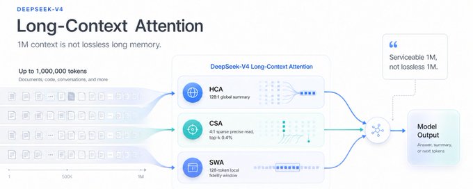
> 1M context is not lossless long memory.DeepSeek-V4 turns attention into three things running in parallel: a 128:1 global summary (HCA), a 4:1 sparse-selection top-k=0.4% precise read (CSA), and a 128-token local-fidelity window (SWA). Each lane handles a different precision regime.KV cache shrinks to 2% of a BF16 GQA8 baseline. The cost: MRCR 8-needle accuracy drops from 0.94 at 8K to 0.59 at 1M. An order of magnitude cheaper than V3.2, but still 10 points behind Claude Opus 4.6 (0.93).Below is a component-by-component breakdown of how V4 engineers a "seemingly impossible 1M" into a "routinely serviceable 1M" — and why this design fundamentally cannot replace RAG.
## 1. Two narratives behind the "1M" number
The open-source community now treats context length as a standalone spec, like RAM size. Llama 4 1M, Qwen3 256K, GLM 4.5 400K, DeepSeek-V4 1M — on paper, it looks like just a number, with the implicit assumption that the model "works on contexts of this length the same way it works on short ones."
That's a misread.
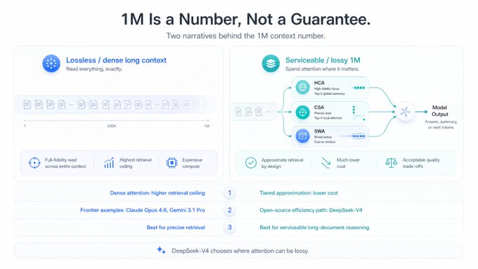
Closed-source frontier labs like Anthropic and Google haven't published their long-context architectures, but when Claude Opus 4.6 scores 92.9 on MRCR 8-needle at 1M and Gemini 3.1 Pro scores 92.4, you can roughly infer they're using something close to dense — paying engineering cost for a high retrieval ceiling.
DeepSeek-V4 takes the opposite approach: accept that attention has to be lossy at 1M, then place the losses where the model is least sensitive.
After walking that road, V4-Pro hits 83.5 on MRCR 8-needle at 1M, V4-Flash hits 49.4, and V3.2 simply cannot be deployed at that length. V4's "1M" is not a "lossless 1M" — it's "a 1M that becomes serviceable under acceptable quality cost."
That's the anchor for the entire piece. Following V4's architecture diagram layer by layer, this judgment will only get more concrete.
## 2. The numbers hook: what 27%/10% and 10%/7% really mean
The paper's core pitch is two pairs of percentages:
- V4-Pro vs V3.2 @ 1M: single-token inference FLOPs down to 27%, KV cache down to 10%
- V4-Flash vs V3.2 @ 1M: single-token inference FLOPs down to 10%, KV cache down to 7%
- vs BF16 GQA8 baseline @ 1M: V4 series KV cache ≈ 2% of baseline
These numbers are honest — V3.2 already incorporates DSA, so this is incremental on top of an already optimised baseline. But three footnotes get glossed over.
Footnote 1 · The comparison baseline is V3.2, not vanilla attention. V3.2 vs Llama-style dense attention already has a 3–5x gap on its own. So "V4 saves 10x over V3.2" is by no means equivalent to "V4 saves 30x over dense attention." The accurate framing is "on top of an already-sparsified baseline, we squeeze another order of magnitude."
Footnote 2 · The "1/3 speedup from FP4 × FP8" is a future-hardware option, not realised today. On H100 / H200 / B200, FP4 × FP8 peak FLOPs are identical to FP8 × FP8. The paper's exact wording is "theoretically can be 1/3 more efficient on future hardware" — a forward-looking note for B300 / NVFP4-class hardware. Today's deployments don't get it.
Footnote 3 · "2% KV cache vs BF16 GQA8" is the product of four compression layers, not a single trick.
1. Sequence-dimension compression (CSA m=4, HCA m'=128)
2. K and V sharing (MLA-style, half off)
3. BF16 → FP8 (non-RoPE dimensions, another ~50% off)
4. Indexer KV in FP4 (one more notch down)
Multiplied together, you get 2%. Each layer pays its own information-loss cost.
Treat these numbers as facts, but remember they're achieved under degraded retrieval quality. The MRCR 8-needle curve in Figure 9 — sliding from 0.94 at 8K all the way to 0.59 / 0.49 at 1M — is the real shape of the cost.
## 3. Architecture overview: V4 attention is a three-lane parallel retrieval system
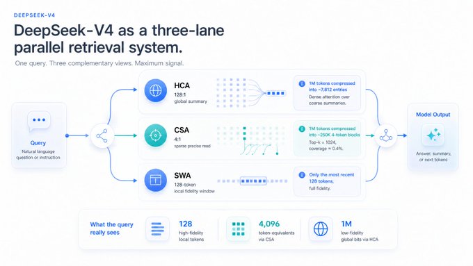
Before unpacking CSA/HCA individually, establish the global picture. Each attention layer in V4 (excluding the first two) is actually a three-lane parallel structure. At every layer, a query simultaneously taps three information channels:
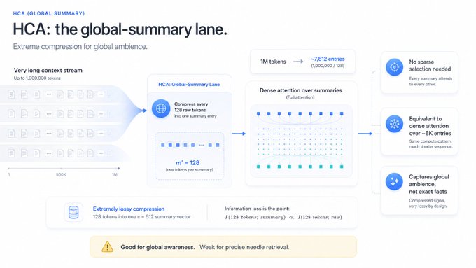
① HCA (global-summary lane)Compression ratio m'=128. 1M tokens compressed into ~7,812 entries; each entry is a lossy summary of 128 raw tokens. Query attends densely to all of them. Covers the entire 1M (global), but each point is severely degraded in precision.
② CSA (sparse-precise-read lane)Compression ratio m=4. 1M tokens compressed into ~250K 4-token blocks. The Lightning Indexer scores all of them and lets the query attend only to the top-k=1024 most relevant ones. Coverage = the entire 1M, but only ~0.4% is actually read by the query.
③ SWA (local-fidelity lane)No compression. The most recent 128 tokens' K/V were kept in full fidelity. Only the last 128 tokens, but completely preserved.
The information budget the query actually "sees":
Lane High-fidelity bits Note SWA 128 token-equivalents · 100% fidelity local context CSA 1,024 × 4 = 4,096 token-equivalents · 4:1 lossy indexer-picked precise-read region HCA 7,812 × 128 = full 1M tokens · 128:1 lossy global ambience
Total ≈ 4,224 high-fidelity bits + 1M low-fidelity bits = "sparse precise read + blurry global view."
This is the anchor for everything that follows. None of the three lanes can stand alone — SWA only sees 128 tokens; whatever CSA misses globally is gone forever; HCA's 128:1 compression is too information-sparse for precise retrieval. That's exactly why V4 has to run all three in parallel rather than picking one.
## 4. CSA: compression + sparse selection, the precise-read lane
4.1 The two-step design
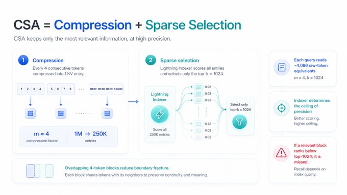
CSA (Compressed Sparse Attention) thins information in two steps:
1. Step 1 — compression: every m=4 consecutive tokens' hidden states are compressed into 1 KV entry using learned softmax weights. 1M tokens → 250K entries.
2. Step 2 — sparse selection: an independent Lightning Indexer scores all 250K entries; the query attends only to the top-k=1024.
That's the two-layer saving from "compression + sparsity." Each query effectively reads 1024 × 4 = 4096 raw-token equivalents — but those 4096 tokens are picked by the indexer based on what it thinks is most relevant, not what the query actually needs. If the indexer picks the wrong one, the blocks the query genuinely needs are simply gone.
4.2 The Lightning Indexer: a cheap top-k decision-maker
The Lightning Indexer was introduced in V3.2 and inherited directly by V4. It's essentially a very thin, independent attention sub-network used only for scoring, never participating in the final output:
- Independent indexer KV (one per 4 tokens, head dim only 128)
- FP4 dot products — even cheaper than the main attention's FP8
- ReLU activation followed by top-k
This is a beautiful engineering decoupling: "deciding where to look" and "what to look at" are separated. But it carries a fundamental risk: the indexer's ranking quality determines the upper bound of the main attention. If the indexer ranks a truly relevant entry at position 1100, the top-k=1024 query will never see it.
The paper does not provide an indexer-accuracy ablation. On MRCR at 1M, V4's top-k coverage is 1024 / 250000 ≈ 0.41% — meaning the indexer must rank each of the 8 needles' compressed blocks within the top-1024. If even one falls outside, the 8-needle task loses one needle.
4.3 Overlap compression: V4's small innovation on CSA
The genuinely new piece in CSA relative to V3.2's DSA is overlap compression: two sets of KV (C^a, C^b) are produced simultaneously, covering staggered 4-token blocks, then cross-block softmax is applied over a wider window.
The benefit is mitigating "information fracture at block boundaries" — under naive compression, if a needle straddles two 4-token blocks, its semantics are split. Overlap compression amounts to a 50%-stride convolutional perspective.
The cost is concrete: pre-compression KV memory doubles (two sets of K, V instead of one), and the CSA layer's parameter count doubles. The cost gets absorbed by §3.5.3's contextual parallelism, but training-time activation memory pressure is real.
## 5. HCA: heavy compression + full dense, the coarse-grained global summary
5.1 A counterintuitive design choice
HCA (Heavily Compressed Attention) takes the opposite philosophy from CSA:
Dimension CSA HCA Compression ratio m = 4 m' = 128 Compression style Overlap (two KV sets) Non-overlap (single KV set) Sparse selection? Yes (top-k=1024) No, full dense Indexer needed? Yes No Tokens condensed per entry 4 128
The interesting questionis: why does HCA dare togo "compress and then dense-attend directly," with no sparse selection?
The answer is in the numbers. After m'=128 compression, 1M tokens shrink to 1,000,000 / 128 ≈ 7,812 entries. 7,812 KVs is well within the budget of dense attention — equivalent to dense attention on an 8K context, roughly 4 GFLOPs on an H100. Totally fine.
So HCA's core trade is: "trade extreme compression for the elimination of sparse-selection complexity." CSA is "light compression + selection"; HCA is "heavy compression + view all." Both pull attention out of the O(N²) regime into a serviceable range, but through entirely different mechanisms.
5.2 The limit of information density
m'=128 means each compressed entry must cram 128 raw tokens' semantics into a c=512-dimensional vector. Given that the original hidden state is also d=4096~7168 dimensions, 128 tokens × 7168 dim = ~917K dimensions of information squeezed down to 512 — a compression ratio of 1800:1.
This is the lossiest stage in V4's architecture. HCA entries are destined to capture "global ambience" rather than "specific facts." They can tell the query "what region X of the 1M context is generally about," but cannot precisely say "at token position 543,217, the specific name of variable X is Y."
This observation maps directly onto Figure 9's MRCR curve: the drop at ≥256K on precise-retrieval tasks can be read almost literally as "HCA's semantic granularity can't keep up with needle-level precision."
## 6. Sliding Window: the local-safety net for when compression fails
6.1 A patched-on design
Looking at CSA + HCA alone, there's a serious problem: causality requires the query to not attend to its own compressed block (otherwise it leaks future-token information).
This means: the most recent stretch of tokens including the query itself is invisible to both CSA and HCA — CSA can't see its own 4-token block; HCA can't see its own 128-token block.
But in language modelling, the most recent few tokens are precisely the most critical signal for next-token prediction. The contradiction has to be resolved, so V4 adds a third lane: Sliding Window Attention (SWA), in which each query additionally attends to the K/V of the most recent n_win = 128 uncompressed tokens.
6.2 An equality that's not a coincidence
Notice a design detail: n_win = m' = 128.
These two numbers being equal isn't accidental — SWA's window size is exactly HCA's compression ratio, meaning SWA covers exactly the "current HCA block" range that HCA can't see due to causality.
So engineering-wise, the three lanes are in strict complementary division of labour:
- SWA covers the most recent 128 tokens (the current HCA block's range)
- HCA covers all earlier compressed HCA blocks (start → ~current - 128)
- CSA picks top-k=1024 from all 4-token compressed blocks, no positional restriction
This division makes one thing clear: pure compressed attention is engineering-infeasible without an uncompressed local window as a fallback. SWA is an "elegant patch," but it's still a patch — its very existence acknowledges that "compression has limits."
## 7. Attention Sink: making "look at nothing" a legitimate option
This trick comes from StreamingLLM (Xiao et al. 2024) and was also used in GPT-OSS. V4's implementation: each attention head has a learnable scalar z'_h added to the softmax denominator.
Result: attention weights no longer have to sum to 1. They can be 0.7, 0.3, or close to 0.
This trick matters especially under sparse attention. Sometimes none of CSA's top-k=1024 selected entries are actually relevant — say the query is "what's the value of this variable?" but the indexer dropped all the relevant blocks. Without a sink, softmax forces attention to spread evenly across those 1024 irrelevant entries, generating massive noise. With a sink, the model can learn "I don't care about any of these 1024 — let attention flow entirely to the sink," and the layer's output is barely affected.
> What sink really means: it gives an attention layer the legitimate option to opt out of the current layer. Without it, sparse-attention failure mode is quietly emitting wrong signal; with it, failure mode becomes emitting near-zero signal and letting the next layer recover. Former is silent corruption, latter is graceful degradation.
## 8. Partial RoPE: position encoding done with care
V4 uses partial RoPE on CSA / HCA — applying RoPE only to the last 64 dimensions of query and KV vectors, leaving the rest position-agnostic. This dates back to V2's MLA and is inherited by V4.
But V4 adds an interesting little detail: inverse RoPE on the output side.
The problem: CSA / HCA's KV is K=V shared (MQA-style); attention output is Σ s_j × V_j. If the last 64 dimensions of V_j carry absolute position encoding (pos j), then Σ s_j × V_j mixes RoPEs across all different positions into a "weighted sum of positions" — neither absolute nor relative, basically noise.
V4's fix: on the output side, rotate the attention output with RoPE at position = -i. This makes the output's "effective position" become j - i = -dist, meaning each V_j's contribution to the output is re-encoded by the query-key distance, automatically converted into relative position encoding.
I haven't seen this trick in any other paper. Mathematically, it's elegant — it resolves the inherent contradiction of "K=V sharing + absolute RoPE." But again, the V4 paper provides no ablation; we just have to trust that "it works fine."
## 9. The cost in quality: the honest curve in Figure 9
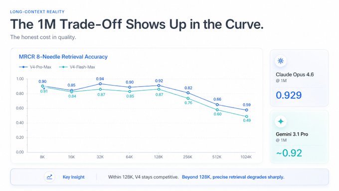
Set the architecture aside and look at the data. Figure 9 plots V4's MRCR 8-needle retrieval accuracy across context length:
Context 8K 16K 32K 64K 128K 256K 512K 1024K
V4-Pro-Max 0.90 0.85 0.94 0.90 0.92 0.82 0.66 0.59
V4-Flash-Max 0.91 0.84 0.87 0.85 0.87 0.76 0.60 0.49
For comparison, frontier models on MRCR 1M 8-needle:
- Claude Opus 4.6: 0.929
- Gemini 3.1 Pro: ~0.92 (paper-reported)
- V4-Pro-Max: 0.835 (Table 7)
A few facts worth surfacing:
Fact 1: Within 128K, V4-Pro is close to the frontier (0.92 vs 0.93). 1M is where divergence actually shows up — there V4 trails Claude by 9–10 absolute points.
Fact 2: V4-Pro at 1M (0.59) beats V4-Flash (0.49). Bigger total params + a larger top-k (1024 vs 512) directly help with long-context retrieval — Pro has twice as many "high-fidelity bits" as Flash.
Fact 3: Figure 9's curve has a "rebound" at 32K, hitting 0.94, then declines monotonically. The 0.59 at 1M is 34 points lower than 0.90 at 8K — that's the concrete number behind "the quality cost of 1M context."
The paper's wording is worth quoting:
> retrieval performance remains highly stable within a 128K context window. While a performance degradation becomes visible beyond the 128K mark, the model's retrieval capabilities at 1M tokens remain remarkably strong compared to both proprietary and open-source counterparts.
"Remarkably strong compared to ... counterparts" is true — among open-source peers, V4 does lead. But what gets glossed over is the drop from 0.92 to 0.59 after 128K. For a rigorous technical reader, that curve is the clearest evidence of V4's engineering trade-off.
## 10. A counterintuitive observation: V4 actually scores higher at 1M than at 128K?
Note this set of numbers from Table 7:
MRCR 8-needle 128K MRCR 8-needle 1M
V4-Pro-Max 78.6 83.5 V4-Pro 78.4 81.0
1M scores higher than 128K?
This contradicts the trend in Figure 9 (same task, more lengths) — Figure 9 is monotonically decreasing. The two numbers in Table 7 are "official highlight scores at specific lengths," and they show 1M > 128K.
The paper doesn't explain the anomaly. Two guesses:
1. Training distribution: V4's late-stage long-context training concentrates around 1M; the model is "more familiar" with that length. 128K is just a "transit point" in the training schedule and may not have been fully consolidated.
2. HCA's sweet spot: a 1M sequence under m'=128 compression yields 7,812 dense entries — exactly HCA's design optimum. A 128K sequence only produces 1,000 entries, which is too sparse and doesn't let HCA's dense advantage shine.
Either way, the anomaly tells us one thing: V4's long-context capability is "trained for 1M," not "generic across lengths." If your real workload is at 200K~500K, you may not be hitting the sweet spot the paper highlights.
## 11. Putting all the pieces back together
The previous 10 sections compressed into one sentence:
> V4's attention isn't attention — it's a composite retrieval system of "lossy compression + sparse retrieval + local fidelity + explicit abstention." At every layer, a query simultaneously consults three views at different granularities (SWA local, CSA precise, HCA global), relying on the indexer's ranking quality, the attention sink's "give up" mechanism, and partial RoPE's position coupling to engineer the "seemingly impossible" 1M into "routinely serviceable."
The real position of this design isn't "innovation" — it's engineering-grade assembly of pre-existing, individually validated components:
- Lightning Indexer + top-k: V3.2 DSA
- Latent query / low-rank K=V sharing: V2 MLA
- Partial RoPE: V2 onward
- Sliding Window: Mistral / Gemma mainstream
- Attention Sink: StreamingLLM, GPT-OSS
- Compress + dense interleaving: Native Sparse Attention lineage
V4's real contribution is the engineering composition + end-to-end 1M serviceability: making these components coexist in a stably trained 32T-token, 1.6T-parameter MoE, paired with custom KV cache management, sparse-attention kernels, and contextual-parallelism training infrastructure.
It's solid systems work, but it isn't a "lossless 1M breakthrough" — it's an engineering victory of "pulling the marginal cost of 1M context into an acceptable range, at the cost of acceptable precise-retrieval degradation."
## 12. Takeaways for the reader
When an open-source model claims 1M context
- Ask whether the attention is dense. If not, it's 1M is a lossy 1M.
- Ask for MRCR 1M 8-needle scores. 0.85+ is frontier-tier; 0.5–0.6 means "runnable but not for precise retrieval."
- Ask for the compression ratio. HCA-style 128:1 compression dooms certain precision tasks — that's not something "more training" can fix.
When designing long-context applications
- Don't use V4 for strict needle retrieval. Use Claude Opus 4.6 / Gemini 3.1 Pro, or just put RAG in front.
- V4's sweet spot is long-document reasoning (e.g., CorpusQA, where V4-Pro-Max scores 33.6 vs Gemini's 35.4) — tasks that need "global ambience + local detail" rather than point-to-point precise matching.
- Good fits: large codebase analysis, multi-document summarisation, and agent long-trajectory maintenance.
- Bad fits: legal-clause retrieval, extracting specific numbers / named entities from medical literature, citing precise timestamps in long transcripts.
When doing architecture research
- Lossy long-context is now a consensus path. Native Sparse Attention, MLA, DSA, Linear Attention, State-Space hybrids — they're all on this path, just varying the compression/sparsity/state ratio.
- V4's real lesson is "tiering": different layers use different compression strategies (CSA / HCA interleaved); different lanes use different precision (SWA full + CSA dense + HCA sparse). This kind of hybrid clearly outperforms any single strategy.
- Three open questions worth pursuing: How does the indexer's top-k ranking accuracy ablate? It's the bottleneck on CSA's ceiling.
Is HCA's m'=128 the empirical optimum, or would m'=64 / 256 also work? The paper doesn't sweep this curve.
The attention weight allocation across the three lanes is learned — could the sink already be "switching off the entire HCA lane" in some layers? That would imply HCA's actual contribution is overstated.
## 13. Closing
"1M context" as a spec line has been refreshed repeatedly during the 2025–2026 open-model race. V4's real contribution is that it wrote down, for the first time, a complete answer to "how is 1M actually built" — not "we widened the attention window," but "we shredded attention with five different compression/selection / windowing mechanisms, each handling the granularity it's best suited for."
That kind of transparency deserves encouragement. But readers — especially engineering readers — need to see the architectural cost hiding behind the spec numbers:
- 1M's KV cache is only 2% of BF16 GQA8 because information has been squeezed through four compression layers
- 1M's FLOPs are only 27% of V3.2's because attention has degenerated from O(N²) into a "tiered approximation, roughly O(N · log N)"
- 1M's retrieval accuracy slid from 0.94 at 8K to 0.59 because this approximation has a precision ceiling, and that ceiling won't be cured by training data
Next time someone tells you "1M context models are here, RAG is dead," send them the curve from Figure 9 — the one going from 0.94 down to 0.59.
1M context ≠ lossless long memory.
It's an engineering-tradeoff victory, and it's an honest disclosure: for some tasks, you still need RAG, you still need dense attention, you still need other external memory systems.
V4 didn't solve the long context. V4 just pushed "the serviceable boundary of long context" considerably further. That's already plenty.
References: DeepSeek-AI, "DeepSeek-V4: Towards Highly Efficient Million-Token Context Intelligence" (2026); Hugging Face Blog, "DeepSeek-V4: a million-token context that agents can actually use"; NVIDIA Developer Blog, "Build with DeepSeek V4 Using NVIDIA Blackwell"; Andrew Lukyanenko, "DeepSeek-V4 Review: Why Million-Token Context Needs Efficient Attention" (Medium, Apr 2026); BigDataBoutique, "Needle in haystack? Optimizing Retrieval and RAG over Long Context Windows"; Liu et al., "Lost in the Middle: How Language Models Use Long Contexts"; Xiao et al., "Efficient Streaming Language Models with Attention Sinks" (StreamingLLM).
## 相关链接
- [GoGoNN](https://x.com/hhjjjFinFin)
- [@hhjjjFinFin](https://x.com/hhjjjFinFin)
- [8.2K](https://x.com/hhjjjFinFin/status/2048773590942970275/analytics)
- [Upgrade to Premium](https://x.com/i/premium_sign_up)
- [10:37 PM · Apr 27, 2026](https://x.com/hhjjjFinFin/status/2048773590942970275)
- [8,277 Views](https://x.com/hhjjjFinFin/status/2048773590942970275/analytics)
---
*导出时间: 2026/4/28 15:26:44*