The Math of RL: From Policy Gradients to PPO and GRPO

Harsh Bhatt 2026-08-31 17.7 KB 56K 567 𝕏 文章列表

本文深入讲解强化学习的数学原理，重点推导策略梯度、REINFORCE、PPO 和 GRPO 等算法。作者首先介绍 RL 的基本流程（Agent、环境、奖励、策略），并通过数学推导得到策略梯度估计器。随后指出原始策略梯度存在的高方差和偏置问题，引入 REINFORCE 算法进行改进。文章还结合 RLHF 和 RLVR 在大语言模型训练中的应用背景，说明 RL 在 LLM 对齐及数学、编程能力提升中的重要作用，帮助读者理解现代 LLM 强化学习训练的底层机制。

强化学习策略梯度 PPO GRPO REINFORCE RLHF 数学推导 LLM训练

# The Math of RL: From Policy Gradients to PPO and GRPO **作者**: Harsh Bhatt **日期**: 2026-08-30T11:14:53.000Z **来源**: [https://x.com/harshbhatt7585/status/2094021031551766970](https://x.com/harshbhatt7585/status/2094021031551766970) --- ![Image](/doc/5585/image/img_343164663ea0.jpg) Reinforcement Learning is becoming very popular since last few years especially in LLMs with the techniques like RLHF (Reinforcement Learning Human Feedback) and RLVR (Reinforcement Learning Verifiable Rewards). RL got the very high attention when DeepMind built and trained AlphaGo, but there came a period when shift moved towards unsupervised technique adversarial loss with GANs, semi-supervised learning with transformers, but as LLMs uplifted the entire deep learning, researchers looked backed into RL. Because of RL we can able to align LLMs using RLHF and make them expert in skills like math and coding through RLVR. In this blog, we will go deep into mathematics of RL,` derive RL algorithms like Policy Gradient, PPO, GRPO and other variants. First let's understand RL in depth, in simple words, it's a way to train an AI model through tiral and error process without needing an extremely supervised dataset. This is the simplest demonstration of RL pipeline: Agent --> Environment --> Rewards --> Update --> Repeat RL training has three major components which we need to understand: 1. Action (at) --> what action agent took in timestep t 2. State (st) --> Which state agent took is in timestep t. 3. Rewards (rt) --> Rewards at timestep t. 4. Policy --> Policy decides which action to take at state t. Agent interacts with ENV, and get rewarded or penalized by it based on their action, by iterating many times using learning algorithm, it learns to take better action. Rewards are the signal for learning algorithm and it pushes to take those action which are high rewards. In an trajactory, the objective is to collect as many rewards and avoid any penalized rewards like in chess, the more games the agent wins the more rewards it gets, in Atari the more score it make the more rewards it gets, Now the policy during learning changes the distribution and makes the high probability of those action which are more likely to give high rewards, well how can we discover which action are good and which action aren't? It comes from Experience, the more diverse experience an agent has the more it will know what works and what not, and that's what we do in RL. RL is a way to learn through experiences, not through any pre-defined dataset. Let's define policy: $$ [ \pi(a \mid s) = P(a_t = a \mid s_t = s) ] $$ > Given the current state s_t, what is the probability of choosing action a_t? Agent's goal: Maximize the rewards. $$ \pi^* = \arg\max_{\pi} \mathbb{E}_{\tau \sim p_\pi(\tau)} \left[ \sum_{t=0}^{T} r(s_t, a_t) \right] $$ This is the expected total reward of a policy. We sample trajectories from the probability distribution created by the policy, then sum the rewards over time, and take the average. Now our agent know what it has to do, collect as many as rewards in a Trajactory. Our policy most probably will be a Neural Network, which could be transformers, RNNs, etc structure. We will do forward pass which will spits out the action from action space. The agent then use that action to take step in the environment, and get rewards. Now to train the model we need to do backward pass to train this policy, so it will adjust its distribution to produce the actions which can collect high rewards. Think about what is the objective, what we are maximizing? yes, Rewards. Which is: $$ \theta^* = \arg\max_{\theta} J(\theta) = \arg\max_{\theta} \mathbb{E}_{\tau \sim p_\theta(\tau)} \left[ \sum_{t=0}^{T} r(s_t, a_t) \right] $$ We have to calculate the gradient of the J of theta, that's what backpropogation do. $$ \nabla_\theta J(\theta) = \nabla_\theta \mathbb{E}_{\tau \sim p_\theta(\tau)} \left[ \sum_{t=0}^{T} r(s_t, a_t) \right] $$ Let's compute the gradient of this: $$ \mathbb{E}{\tau \sim p\theta(\tau)} \left[ r(\tau) \right] ] $$ where the total reward of a trajectory is: $$ \sum_{t=0}^{T} r(s_t, a_t) ] $$ Writing the expectation as an integral over trajectories: $$ \int p_\theta(\tau) r(\tau) d\tau ] $$ Now we take the gradient of it. $$ \nabla_\theta \int p_\theta(\tau) r(\tau) d\tau ] $$ Since the reward function does not directly depend on theta, we move the gradient inside: $$ \int \nabla_\theta p_\theta(\tau) r(\tau) d\tau $$ Now we use the log-derivative trick: $$ p_\theta(\tau) \nabla_\theta \log p_\theta(\tau) $$ Substituting this back: $$ \int p_\theta(\tau) \nabla_\theta \log p_\theta(\tau) r(\tau) d\tau $$ This can be written again as an expectation: $$ \mathbb{E}{\tau \sim p\theta(\tau)} \left[ \nabla_\theta \log p_\theta(\tau) r(\tau) \right] $$ Now expand the trajectory probability: $$ p(s_0) \prod_{t=0}^{T} \pi_\theta(a_t \mid s_t) p(s_{t+1} \mid s_t, a_t) $$ Taking log on both sides, to simplify this from product to addition: $$ \log p(s_0) + \sum_{t=0}^{T} \log \pi_\theta(a_t \mid s_t) + \sum_{t=0}^{T} \log p(s_{t+1} \mid s_t, a_t) ] $$ The environment transition does not depend on theta, and the initial state distribution p(s_0) also does not depend on theta. Therefore, their gradients are zero: $$ \sum_{t=0}^{T} \nabla_\theta \log \pi_\theta(a_t \mid s_t) ] $$ Substituting this into the policy gradient expression: $$ \mathbb{E}{\tau \sim p\theta(\tau)} \left[ \left( \sum_{t=0}^{T} \nabla_\theta \log \pi_\theta(a_t \mid s_t) \right) r(\tau) \right] $$ Since: $$ \sum_{t=0}^{T} r(s_t, a_t) $$ We get: $$ \mathbb{E}{\tau \sim p\theta(\tau)} \left[ \left( \sum_{t=0}^{T} \nabla_\theta \log \pi_\theta(a_t \mid s_t) \right) \left( \sum_{t=0}^{T} r(s_t, a_t) \right) \right] $$ This is the basic policy gradient estimator. This means that we increase the probability of actions that lead to high future reward, and decrease the probability of actions that lead to low future reward. But here every action getting the the total from timestep 0 to T, see the summation of the Reward. $$ \left( \sum_{t=0}^{T} r(s_t, a_t) \right) $$ So what will happen, let's suppose at a3 it got -5 reward, and a1 and a2 are 5 and 10. $$ r = r1 + r3 + r3 $$ $$ r = 5 + 10 - 5 = 10 $$ during the learning, it will promote the action taken at a3 given the total with of previous reward still high inspite of getting -5 at a3, And this adds a biasness and noise that's why better way is remove the previous reward during each action step of reward computation, here's the better way mentioned in policy gradient: $$ \left( \sum_{t=t'}^{T} r(s_t, a_t) \right) $$ See it starts from t=t' , now the full equation will look like this: $$ \mathbb{E}{\tau \sim p\theta(\tau)} \left[ \left( \sum_{t=0}^{T} \nabla_\theta \log \pi_\theta(a_t \mid s_t) \right) \left( \sum_{t=t'}^{T} r(s_t, a_t) \right) \right] $$ This is also called REINFORCE which was introduced in 1992 in the paper "[Simple Statistical Gradient-Following Algorithms for Connectionist Reinforcement Learning](https://link.springer.com/article/10.1007/BF00992696?utm_source=chatgpt.com)" by Ronald J. Williams The problem with REINFORCE was that, reward of each step directly used as training signal, as a result sometimes the model get's high reward so the model adjust its parameter in the direction of reward and then in the next consecutive turn the model gets negative reward and then again the model adjust its parameters away from that direction, this sudden changes in reward signals creates a high variance and confuses the model a lot in learning. To Fix this, we can redefine our training signal to the model, what if we use average reward across trajactories? This is good idea, but we also have to give reward to each step of the action to give them better feedback so instead of this we can give training signal whether the current reward is better than average reward or not? if it is not then it's not worth hyping up, and telling the model to go in that direction, if it is better than average reward then its more than our expectation, let's tell the model to go in that direction. $$ b = \frac{1}{N}\sum_{i=1}^{N} r(\tau^{(i)}) $$ b is a baseline here, which computes the mean reward across trajectory. $$ \mathbb{E}{\tau \sim p\theta(\tau)} \left[ \left( \sum_{t=0}^{T} \nabla_\theta \log \pi_\theta(a_t \mid s_t) \right) (r(\tau) - b) \right] $$ We can substract rewards in trajectory with the constant average reward, and this b is unbiased and does not change the gradient, and here's why: $$ E[\nabla_\theta \log p_\theta(\tau)b] = \int p_\theta(\tau)\nabla_\theta \log p_\theta(\tau)b\,d\tau = b\int \nabla_\theta p_\theta(\tau)\,d\tau = b\nabla_\theta\int p_\theta(\tau)\,d\tau = b\nabla_\theta 1 = 0 $$ We also call this "Subtracting of average reward" as Advantage, which tells what either we have negative advantage or positive. $$ A = r(\tau) - b $$ So the final equation of gradient will look like: $$ \mathbb{E}{\tau \sim p\theta(\tau)} \left[ \left( \sum_{t=0}^{T} \nabla_\theta \log \pi_\theta(a_t \mid s_t) \right) A \right] $$ This is the foundation of all RL pipeline like RLHF, RLVR and training RL based agents, all the famous RL methods like PPO, RLHF, GRPO, etc are variations or built on top REINFORCE. Now let's think about this how an Model like LLM trains using RL methods in production and large scale, first let's learn about Off-Policy and On-Policy Method. ## On-Policy Generally in RL training pipeline, our agent take action from policy and interacts with the environment, and training algorithm aligns the model in the direction of better rewards. 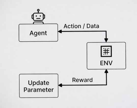![Image](/doc/5585/image/img_e9288dc45193.jpg) At every step the model is collecting its own data by interacting with the environment and using that to train itself, so every step the agent generating data has always from updated policy. This is called On-Policy where we use the same updated policy to collect data for training. ## Off-Policy When the data is generated from different policy than the policy being updated during training, it is called Off-Policy learning. The policy that generates the experience is called the behavior policy, while the policy being updated is called the target policy. For instance, there is a teacher model which is already trained, we can use that to sample the data, and agent can use that as a experience to update the parameters. That's why most of the time off-policy learning is more efficient because we already have data prepared, where as in on-policy the data is generated on the fly while training. 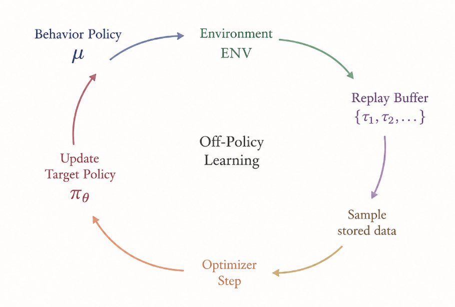![Image](/doc/5585/image/img_c34dbd98ff62.jpg) ## TRPO [Trust Region Policy Optimization](https://arxiv.org/pdf/1502.05477) is a major upgrade in Policy Gradient, it asked question "Can we estimate the future rewards beforehand and direct our model towards a better state?", To solve this, authors added Value function. Value function simply is a value of a state. Value of a state means how much reward it can get in that state. The value of a state is the expected sum of future rewards an agent will receive, starting from that state and following a policy. $$ V^\pi(s) = \mathbb{E}_{\pi} \left[ \sum_{t=0}^{T} \gamma^t r_t \mid s_0=s \right] $$ If we can predict the the estimate the future rewards the agent can get from a given state, we can redirect the agent to move in the trajectory where there is highest rewards. To get this intuitively, let's take an example: suppose there are 4 states in a trajectory, s1, s2, s3, and s4. $$ s1 --> s2 --> s3 --> s4 $$ The rewards each state respectively have 0, 0, 1 and 1. the Value of each states will be in non-discounted rewards: $$ V(s_1) = 0 + 0 + 1 + 1 = 2 $$ $$ V(s_2) = s2 + s3 + s4 = 0 + 1 + 1 = 2 $$ $$ V(s_3) = s3 + s4 = 1 + 1 = 2 $$ $$ V(s_4) = s4 = 1 $$ 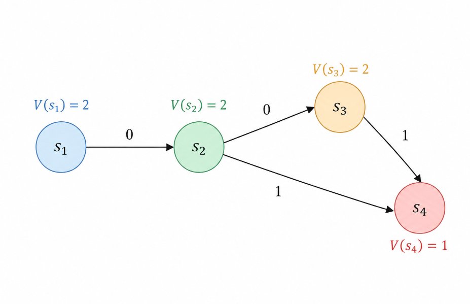![Image](/doc/5585/image/img_532502e38105.jpg) And the add this Value function in Advantage instead of baseline (average reward). So now the equation becomes: $$ \hat{A}_t = \left( \sum_{k=t}^{T} \gamma^{k-t} r_k \right) - V^\pi(s_t) $$ ## PPO [PPO](https://arxiv.org/pdf/1707.06347) is one of the most influential reinforcement learning algorithm created by researchers at OpenAI in 2017. The interesting thing is it was rejected by NIPS at that time. 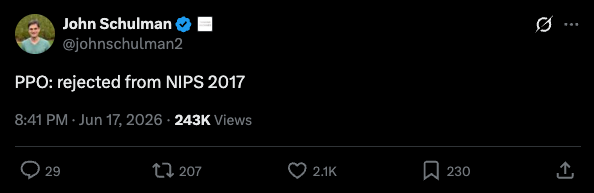![Image](/doc/5585/image/img_4754c607389f.jpg) PPO asked question on how can we reuse collected trajectories for several gradient updates without changing the policy so aggressively that training collapses? It founded a tradeoff between Vanilla policy gradient and TRPO, which helped better balance in variance and stable learning. It introduced new methods like clipping and policy surrogate. PPO performed better than the compared algorithms on almost all continuous-control environments. 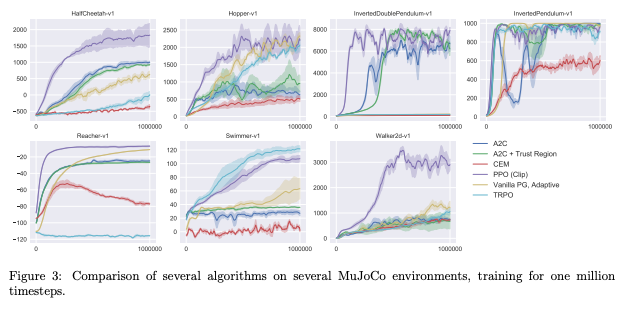![Image](/doc/5585/image/img_930d082cb214.jpg) Vanilla policy-gradient methods often use Monte Carlo future returns, which have low bias but high variance. TRPO uses a learned value function together with GAE to estimate advantages, where the parameter λ balances bias and variance: more bootstrapping gives lower variance but with higher bias, while longer sampled returns give lower bias but higher variance. PPO keeps this GAE-style advantage estimation from TRPO, but replaces TRPO’s complicated KL-constrained update with a simpler clipped surrogate objective. this was we had in TRPO: $$ \max_{\theta} \mathbb{E}_t \left[ \frac{\pi_{\theta}(a_t \mid s_t)}{\pi_{\theta_{\mathrm{old}}}(a_t \mid s_t)} \hat{A}_t \right] $$ $$ \mathbb{E}_t \left[ D_{\mathrm{KL}} \left( \pi_{\theta_{\mathrm{old}}}(\cdot \mid s_t) \parallel \pi_{\theta}(\cdot \mid s_t) \right) \right] \leq \delta $$ PPO: $$ r_t(\theta) = \frac{\pi_{\theta}(a_t \mid s_t)}{\pi_{\theta_{\mathrm{old}}}(a_t \mid s_t)} $$ $$ L^{CLIP}(\theta) = \mathbb{E}_t \left[ \min \left( r_t(\theta)\hat{A}_t,\ clip\left(r_t(\theta),1-\epsilon,1+\epsilon\right)\hat{A}_t \right) \right] $$ It add a clipping method, so if the product of trajectory in reward and Advantage is positive it will use the product itself, if not, it will use clipped version, where the minimum is 1 - epsilon, and max is 1 + epsilon. ## GRPO Group-Relative Policy Algorithm was introduced in DeepSeek-Math Paper in 2024. Because very two network: actor and critic in PPO, As we described above, value function estimates how good the current state is and helps PPO calculate the advantage using methods such as GAE. This works well in small network size models, but for LLMs the critic can itself be another model comparable in size to the policy. That adds the requirement of huge memory and compute, while learning accurate token-level values from mostly sequence-level rewards can also be difficult. DeepSeek's researchers introduced a new variation by removing the critic function and computing the advantage through group of responses LLM. GRPO generates multiple responses to the same prompt and asks “how good was this response compared with the other responses?” For one question (q), GRPO samples a group of (G) outputs: $$ o_1,o_2,\ldots,o_G \sim \pi_{\theta_{\text{old}}}(\cdot|q) $$ Each output receives a reward: $$ r_1,r_2,\ldots,r_G $$ Then GRPO uses the group's reward distribution as its baseline. For outcome-supervised GRPO, the advantage becomes: $$ \frac{ r_i-\operatorname{mean}(r_1,\ldots,r_G) }{ \operatorname{std}(r_1,\ldots,r_G) } $$ So if a response performs better than the group average, it gets positive advantage. If it performs worse than the group average, it gets negative advantage. So, advantage without any value function!! For every token: $$ \frac{ \pi_\theta(o_{i,t}|q,o_{i,<t}) }{ \pi_{\theta_{\text{old}}}(o_{i,t}|q,o_{i,<t}) } $$ and the policy is optimized using: $$ \min \left( r_{i,t}(\theta)\hat A_i, \operatorname{clip} (r_{i,t}(\theta),1-\epsilon,1+\epsilon)\hat A_i \right) $$ GRPO also adds a KL penalty against a reference model: $$ -\beta D_{KL} (\pi_\theta|\pi_{\text{ref}}) $$ so basically it is just PPO without a value function and KL Regularization. Suppose the model generates eight solutions to the same math problem. Instead of training another neural network to predict the value of every solution, GRPO scores all eight, calculates their mean reward, and increases the probability of solutions performing above that mean while decreasing the probability of solutions performing below it. This makes GRPO particularly useful for LLM reasoning tasks where we can cheaply generate several candidate answers and evaluate them using a reward model or a verifiable reward such as whether the final mathematical answer is correct. In DeepSeekMath, GRPO improved GSM8K from 82.9% to 88.2% and MATH from 46.8% to 51.7%, while avoiding PPO's additional critic model. ## Conclusion This article covers the foundation of Reinforcement Learning by deriving the policy gradient methods and showing how they evolved from REINFORCE to TRPO, PPO, and eventually GRPO. the core idea is learning from experience and rewards to make better actions more likely. Understanding this foundation makes modern methods like RLHF and RLVR much easier to understand. I will cover more mordern variants and methods in future article, stay tuned. ## 相关链接 - [Harsh Bhatt](https://x.com/harshbhatt7585) - [@harshbhatt7585](https://x.com/harshbhatt7585) - [33K](https://x.com/harshbhatt7585/status/2094021031551766970/analytics) - [Trust Region Policy Optimization](https://arxiv.org/pdf/1502.05477) - [PPO](https://arxiv.org/pdf/1707.06347) - [Upgrade to Premium](https://x.com/i/premium_sign_up) - [7:14 PM · Aug 30, 2026](https://x.com/harshbhatt7585/status/2094021031551766970) - [33.7K Views](https://x.com/harshbhatt7585/status/2094021031551766970/analytics) - [View quotes](https://x.com/harshbhatt7585/status/2094021031551766970/quotes) --- *导出时间: 2026/8/31 09:29:06* --- ## 中文翻译 # 强化学习的数学：从策略梯度到 PPO 和 GRPO **作者**： Harsh Bhatt **日期**： 2026-08-30T11:14:53.000Z **来源**： [https://x.com/harshbhatt7585/status/2094021031551766970](https://x.com/harshbhatt7585/status/2094021031551766970) --- ![Image](/doc/5585/image/img_343164663ea0.jpg) 近几年来，强化学习变得非常流行，尤其是在大语言模型（LLM）领域，出现了诸如 RLHF（基于人类反馈的强化学习）和 RLVR（基于可验证奖励的强化学习）等技术。当 DeepMind 构建并训练出 AlphaGo 时，强化学习获得了极高的关注度，但随后有一段时间重心转向了无监督技术（如 GAN 的对抗损失）和基于 Transformer 的半监督学习。不过，随着 LLM 带动了整个深度学习的发展，研究人员重新回过头来看强化学习。正是因为强化学习，我们才能通过 RLHF 对齐 LLM，并通过 RLVR 让它们在数学和编程等技能上成为专家。在这篇博客中，我们将深入探讨强化学习的数学原理，推导策略梯度、PPO、GRPO 等算法及其他变体。首先让我们深入理解强化学习。简单来说，它是一种通过试错过程来训练 AI 模型的方法，不需要极度精细监督的数据集。这是强化学习流程最简单的展示：智能体 --> 环境 --> 奖励 --> 更新 --> 重复。强化学习训练有三个需要理解的主要组件：1. 动作 --> 智能体在时间步 t 采取的动作。2. 状态 --> 智能体在时间步 t 所处的状态。3. 奖励 --> 时间步 t 的奖励。4. 策略 --> 策略决定在状态 t 下采取哪个动作。智能体与环境交互，并根据其行为获得奖励或惩罚。通过使用学习算法反复迭代，它学会采取更好的动作。奖励是学习算法的信号，它推动算法采取高奖励的动作。在一条轨迹中，目标是收集尽可能多的奖励并避免任何惩罚性奖励，比如在国际象棋中，智能体赢的棋局越多，获得的奖励就越多；在雅达利游戏中，得分越高，奖励越多。在学习过程中，策略会改变分布，使得那些更可能带来高奖励的动作具有更高的概率。那么我们如何发现哪些动作是好的、哪些动作是不好的呢？这来自经验，智能体拥有的经验越多样，它就越清楚什么有效、什么无效，而这正是我们在强化学习中所做的。强化学习是一种通过经验学习的方法，而不是通过任何预先定义的数据集。让我们定义策略： $$ [ \pi(a \mid s) = P(a_t = a \mid s_t = s) ] $$ > 给定当前状态 s_t，选择动作 a_t 的概率是多少？智能体的目标：最大化奖励。 $$ \pi^* = \arg\max_{\pi} \mathbb{E}_{\tau \sim p_\pi(\tau)} \left[ \sum_{t=0}^{T} r(s_t, a_t) \right] $$ 这是策略的期望总奖励。我们从由策略创建的概率分布中采样轨迹，然后对奖励随时间求和，并取平均值。现在我们的智能体知道它要做什么了：在一条轨迹中收集尽可能多的奖励。我们的策略很可能是一个神经网络，其结构可以是 Transformer、RNN 等。我们进行前向传播，从动作空间中输出动作。然后智能体使用该动作在环境中迈出一步，并获得奖励。现在要训练模型，我们需要进行反向传播来训练这个策略，使其调整分布以产生能收集高奖励的动作。想想目标是什么，我们最大化的是什么？是的，奖励。即： $$ \theta^* = \arg\max_{\theta} J(\theta) = \arg\max_{\theta} \mathbb{E}_{\tau \sim p_\theta(\tau)} \left[ \sum_{t=0}^{T} r(s_t, a_t) \right] $$ 我们需要计算 J(θ) 的梯度，这正是反向传播所做的。 $$ \nabla_\theta J(\theta) = \nabla_\theta \mathbb{E}_{\tau \sim p_\theta(\tau)} \left[ \sum_{t=0}^{T} r(s_t, a_t) \right] $$ 让我们计算这个的梯度： $$ \mathbb{E}{\tau \sim p\theta(\tau)} \left[ r(\tau) \right] ] $$ 其中轨迹的总奖励为： $$ \sum_{t=0}^{T} r(s_t, a_t) ] $$ 将期望写成对轨迹的积分： $$ \int p_\theta(\tau) r(\tau) d\tau ] $$ 现在我们取它的梯度。 $$ \nabla_\theta \int p_\theta(\tau) r(\tau) d\tau ] $$ 由于奖励函数不直接依赖于 θ，我们把梯度移到积分内部： $$ \int \nabla_\theta p_\theta(\tau) r(\tau) d\tau $$ 现在我们使用对数导数技巧： $$ p_\theta(\tau) \nabla_\theta \log p_\theta(\tau) $$ 将其代回： $$ \int p_\theta(\tau) \nabla_\theta \log p_\theta(\tau) r(\tau) d\tau $$ 这可以再次写成期望的形式： $$ \mathbb{E}{\tau \sim p\theta(\tau)} \left[ \nabla_\theta \log p_\theta(\tau) r(\tau) \right] $$ 现在展开轨迹概率： $$ p(s_0) \prod_{t=0}^{T} \pi_\theta(a_t \mid s_t) p(s_{t+1} \mid s_t, a_t) $$ 两边取对数，将乘积简化为加法： $$ \log p(s_0) + \sum_{t=0}^{T} \log \pi_\theta(a_t \mid s_t) + \sum_{t=0}^{T} \log p(s_{t+1} \mid s_t, a_t) ] $$ 环境转移不依赖于 θ，初始状态分布 p(s_0) 也不依赖于 θ。因此，它们的梯度为零： $$ \sum_{t=0}^{T} \nabla_\theta \log \pi_\theta(a_t \mid s_t) ] $$ 将其代入策略梯度表达式： $$ \mathbb{E}{\tau \sim p\theta(\tau)} \left[ \left( \sum_{t=0}^{T} \nabla_\theta \log \pi_\theta(a_t \mid s_t) \right) r(\tau) \right] $$ 由于： $$ \sum_{t=0}^{T} r(s_t, a_t) $$ 我们得到： $$ \mathbb{E}{\tau \sim p\theta(\tau)} \left[ \left( \sum_{t=0}^{T} \nabla_\theta \log \pi_\theta(a_t \mid s_t) \right) \left( \sum_{t=0}^{T} r(s_t, a_t) \right) \right] $$ 这就是基本的策略梯度估计器。这意味着我们提高那些带来高未来奖励的动作的概率，降低那些带来低未来奖励的动作的概率。但在这里，每个动作都获得了从时间步 0 到 T 的总和，看看奖励的求和： $$ \left( \sum_{t=0}^{T} r(s_t, a_t) \right) $$ 那么会发生什么呢？假设 a3 得到了 -5 的奖励，而 a1 和 a2 分别是 5 和 10。 $$ r = r1 + r3 + r3 $$ $$ r = 5 + 10 - 5 = 10 $$ 在学习过程中，尽管 a3 得到了 -5，但由于之前的奖励总和仍然很高，a3 处采取的动作仍会被强化。这就引入了偏差和噪声，因此更好的方法是在计算每个动作步骤的奖励时去掉之前的奖励，下面是策略梯度中提到的更好的方法： $$ \left( \sum_{t=t'}^{T} r(s_t, a_t) \right) $$ 看，它从 t=t' 开始，现在完整的等式看起来是这样的： $$ \mathbb{E}{\tau \sim p\theta(\tau)} \left[ \left( \sum_{t=0}^{T} \nabla_\theta \log \pi_\theta(a_t \mid s_t) \right) \left( \sum_{t=t'}^{T} r(s_t, a_t) \right) \right] $$ 这也被称为 REINFORCE，由 Ronald J. Williams 在 1992 年的论文《[Simple Statistical Gradient-Following Algorithms for Connectionist Reinforcement Learning](https://link.springer.com/article/10.1007/BF00992696?utm_source=chatgpt.com)》中提出。 REINFORCE 的问题在于，每一步的奖励被直接用作训练信号。因此，有时模型获得高奖励，模型就朝奖励的方向调整参数；然后在接下来的连续回合中，模型又获得负奖励，于是再次把参数往那个方向的相反方向调整。这种奖励信号的突变会造成高方差，并在学习过程中让模型非常困惑。为了解决这个问题，我们可以重新定义给模型的训练信号。如果我们使用各条轨迹间的平均奖励会怎样？这是个好主意，但我们还必须给动作的每一步都给出奖励，以便给它们更好的反馈。所以与其这样做，我们可以给出的训练信号是：当前奖励是否优于平均奖励？如果不是，那就不值得 hype，也不该让模型朝那个方向走；如果优于平均奖励，那就超出了我们的预期，那就让模型朝那个方向走。 $$ b = \frac{1}{N}\sum_{i=1}^{N} r(\tau^{(i)}) $$ 这里的 b 是一个基线，它计算各条轨迹间的平均奖励。 $$ \mathbb{E}{\tau \sim p\theta(\tau)} \left[ \left( \sum_{t=0}^{T} \nabla_\theta \log \pi_\theta(a_t \mid s_t) \right) (r(\tau) - b) \right] $$ 我们可以将轨迹中的奖励减去常数平均奖励，而这个 b 是无偏的，不会改变梯度，原因如下： $$ E[\nabla_\theta \log p_\theta(\tau)b] = \int p_\theta(\tau)\nabla_\theta \log p_\theta(\tau)b\,d\tau = b\int \nabla_\theta p_\theta(\tau)\,d\tau = b\nabla_\theta\int p_\theta(\tau)\,d\tau = b\nabla_\theta 1 = 0 $$ 我们也把这个“减去平均奖励”称为优势，它告诉我们优势是负的还是正的。 $$ A = r(\tau) - b $$ 所以最终的梯度方程看起来像： $$ \mathbb{E}{\tau \sim p\theta(\tau)} \left[ \left( \sum_{t=0}^{T} \nabla_\theta \log \pi_\theta(a_t \mid s_t) \right) A \right] $$ 这是所有强化学习流程（如 RLHF、RLVR 以及训练基于强化学习的智能体）的基础。所有著名的强化学习方法，如 PPO、RLHF、GRPO 等，都是 REINFORCE 的变体或在其之上构建的。现在让我们思考一下，像 LLM 这样的模型在生产环境和大规模场景下是如何使用强化学习方法训练的。首先让我们了解 Off-Policy（异策略）和 On-Policy（同策略）方法。 ## On-Policy（同策略）一般来说，在强化学习训练流程中，我们的智能体从策略中采取动作并与环境交互，训练算法使模型朝更好的奖励方向对齐。 ![Image](/doc/5585/image/img_e9288dc45193.jpg) 在每一步，模型都通过与环境交互来收集自己的数据，并用这些数据来训练自己。因此，智能体在每一步生成的数据总是来自更新后的策略。这被称为 On-Policy，即我们使用同一个更新后的策略来收集训练数据。 ## Off-Policy（异策略）当数据是由与训练中正在更新的策略不同的策略生成时，就称为 Off-Policy 学习。生成经验的策略称为行为策略，而被更新的策略称为目标策略。例如，有一个已经训练好的教师模型，我们可以用它来采样数据，而智能体可以将这些数据作为经验来更新参数。这就是为什么大多数时候 Off-Policy 学习效率更高，因为数据已经准备好了；而在 On-Policy 中，数据是在训练过程中实时生成的。 ![Image](/doc/5585/image/img_c34dbd98ff62.jpg) ## TRPO [Trust Region Policy Optimization（信任区域策略优化）](https://arxiv.org/pdf/1502.05477)是策略梯度的一次重大升级。它提出了一个问题：“我们能否预先估计未来的奖励，并引导我们的模型走向更好的状态？”为解决这个问题，作者加入了价值函数。价值函数简单来说就是一个状态的价值。状态的价值意味着在该状态下可以获得多少奖励。一个状态的价值是智能体从该状态出发、遵循某个策略所能获得的未来奖励的期望总和。 $$ V^\pi(s) = \mathbb{E}_{\pi} \left[ \sum_{t=0}^{T} \gamma^t r_t \mid s_0=s \right] $$ 如果我们能预测智能体从给定状态可以获得的未来奖励的估计值，我们就可以引导智能体朝奖励最高的轨迹移动。为了直观地理解这一点，举个例子：假设轨迹中有 4 个状态：s1、s2、s3 和 s4。 $$ s1 --> s2 --> s3 --> s4 $$ 各状态的奖励分别为 0、0、1 和 1。在不折扣奖励的情况下，各状态的价值为： $$ V(s_1) = 0 + 0 + 1 + 1 = 2 $$ $$ V(s_2) = s2 + s3 + s4 = 0 + 1 + 1 = 2 $$ $$ V(s_3) = s3 + s4 = 1 + 1 = 2 $$ $$ V(s_4) = s4 = 1 $$ ![Image](/doc/5585/image/img_532502e38105.jpg) 然后，用这个价值函数代替基线（平均奖励）加到优势中。所以现在等式变成： $$ \hat{A}_t = \left( \sum_{k=t}^{T} \gamma^{k-t} r_k \right) - V^\pi(s_t) $$ ## PPO [PPO](https://arxiv.org/pdf/1707.06347) 是由 OpenAI 的研究人员于 2017 年创建的最具影响力的强化学习算法之一。有趣的是，它当时曾被 NIPS 拒稿。 ![Image](/doc/5585/image/img_4754c607389f.jpg) PPO 提出的问题是：我们如何将收集到的轨迹复用于多次梯度更新，同时又不会过于激进地改变策略而导致训练崩溃？它在朴素策略梯度和 TRPO 之间找到了一种折中，有助于更好地平衡方差与学习的稳定性。它引入了裁剪和代理策略等新方法。 PPO 在几乎所有连续控制环境中都优于所比较的算法。 ![Image](/doc/5585/image/img_930d082cb214.jpg) 朴素策略梯度方法通常使用蒙特卡洛未来回报，其偏差低但方差高。TRPO 使用学习到的价值函数配合 GAE 来估计优势，其中参数 λ 用于平衡偏差和方差：更多的自举会带来更低的方差但更高的偏差，而更长的采样回报则带来更低的偏差但更高的方差。PPO 保留了 TRPO 的这种 GAE 风格的优势估计，但用更简单的裁剪代理目标取代了 TRPO 复杂的 KL 约束更新。这是 TRPO 中的内容： $$ \max_{\theta} \mathbb{E}_t \left[ \frac{\pi_{\theta}(a_t \mid s_t)}{\pi_{\theta_{\mathrm{old}}}(a_t \mid s_t)} \hat{A}_t \right] $$ $$ \mathbb{E}_t \left[ D_{\mathrm{KL}} \left( \pi_{\theta_{\mathrm{old}}}(\cdot \mid s_t) \parallel \pi_{\theta}(\cdot \mid s_t) \right) \right] \leq \delta $$ PPO： $$ r_t(\theta) = \frac{\pi_{\theta}(a_t \mid s_t)}{\pi_{\theta_{\mathrm{old}}}(a_t \mid s_t)} $$ $$ L^{CLIP}(\theta) = \mathbb{E}_t \left[ \min \left( r_t(\theta)\hat{A}_t,\ clip\left(r_t(\theta),1-\epsilon,1+\epsilon\right)\hat{A}_t \right) \right] $$ 它加入了一种裁剪方法：如果轨迹奖励与优势的乘积为正，就使用该乘积本身；否则，就使用裁剪后的版本，其中最小值为 1 - ε，最大值为 1 + ε。 ## GRPO 组相对策略算法由 DeepSeek-Math 论文于 2024 年提出。由于 PPO 中有两个网络：行动者和评论家。正如上文所述，价值函数估计当前状态的好坏，并帮助 PPO 使用 GAE 等方法计算优势。这在小型网络模型中效果很好，但对于 LLM 来说，评论家本身可能是另一个与策略模型规模相当的模型。这带来了巨大的内存和算力需求，而从主要是序列级别的奖励中学习精确的 token 级别价值也很困难。DeepSeek 的研究人员通过去掉评论家函数、通过 LLM 的一组回答来计算优势，提出了一种新的变体。 GRPO 对同一个提示生成多个回答，并问“这个回答与其他回答相比怎么样？” 对于一个问题，GRPO 采样一组（G 个）输出： $$ o_1,o_2,\ldots,o_G \sim \pi_{\theta_{\text{old}}}(\cdot|q) $$ 每个输出获得一个奖励： $$ r_1,r_2,\ldots,r_G $$ 然后 GRPO 使用该组的奖励分布作为基线。对于结果监督的 GRPO，优势变为： $$ \frac{ r_i-\operatorname{mean}(r_1,\ldots,r_G) }{ \operatorname{std}(r_1,\ldots,r_G) } $$ 所以，如果一个回答的表现优于组平均值，它就获得正优势；如果表现差于组平均值，它就获得负优势。所以，无需任何价值函数的优势！！对于每个 token： $$ \frac{ \pi_\theta(o_{i,t}|q,o_{i,<t}) }{ \pi_{\theta_{\text{old}}}(o_{i,t}|q,o_{i,<t}) } $$ 并使用下式优化策略： $$ \min \left( r_{i,t}(\theta)\hat A_i, \operatorname{clip} (r_{i,t}(\theta),1-\epsilon,1+\epsilon)\hat A_i \right) $$ GRPO 还增加了针对参考模型的 KL 惩罚： $$ -\beta D_{KL} (\pi_\theta|\pi_{\text{ref}}) $$ 所以基本上它就是没有价值函数的 PPO，外加 KL 正则化。假设模型对同一个数学问题生成八个解答。GRPO 不再训练另一个神经网络来预测每个解答的价值，而是对全部八个解答打分，计算它们的平均奖励，并提高表现高于平均值的解答的概率，同时降低表现低于平均值的解答的概率。这使得 GRPO 在 LLM 推理任务中特别有用，因为在这些任务中我们可以低成本地生成多个候选答案，并使用奖励模型或可验证奖励（例如最终的数学答案是否正确）来评估它们。在 DeepSeekMath 中，GRPO 将 GSM8K 从 82.9% 提升至 88.2%，将 MATH 从 46.8% 提升至 51.7%，同时避免了 PPO 额外的评论家模型。 ## 结论本文通过推导策略梯度方法，展示了它们如何从 REINFORCE 演进到 TRPO、PPO，最终到 GRPO，涵盖了强化学习的基础。其核心思想是从经验和奖励中学习，使更好的动作更有可能被采取。理解了这一基础，就能更容易地理解 RLHF 和 RLVR 等现代方法。我将在未来的文章中介绍更多现代变体和方法，敬请期待。 ## 相关链接 - [Harsh Bhatt](https://x.com/harshbhatt7585) - [@harshbhatt7585](https://x.com/harshbhatt7585) - [33K](https://x.com/harshbhatt7585/status/2094021031551766970/analytics) - [Trust Region Policy Optimization](https://arxiv.org/pdf/1502.05477) - [PPO](https://arxiv.org/pdf/1707.06347) - [Upgrade to Premium](https://x.com/i/premium_sign_up) - [7:14 PM · Aug 30, 2026](https://x.com/harshbhatt7585/status/2094021031551766970) - [33.7K Views](https://x.com/harshbhatt7585/status/2094021031551766970/analytics) - [View quotes](https://x.com/harshbhatt7585/status/2094021031551766970/quotes) --- *导出时间: 2026/8/31 09:29:06*

相关文档