Cerebras 如何部署万亿参数前沿模型 Sarah Chieng 2026-10-23 9.9 KB 282.4K 816 ☆ 收藏 𝕏 文章列表 Cerebras 团队详细介绍了如何在 WSE-3T 晶圆级芯片上部署万亿参数大模型。以 3 万亿参数的开源模型 Kimi K3 为例,团队通过 4-bit 权重量化和 8-bit KV 缓存计算每层约 16 GB 的显存需求,将模型切分到 59 片晶圆上:每个 dense 层独占一片晶圆,每片可放两个 linear-attention 层。晶圆间通过以太网 RDMA 传递激活值,权重无需移动。系统以流水线方式运行,各阶段可同时处理不同请求和微批次,从而实现 1000-2000+ tokens/秒的推理速度。 Cerebras推理部署万亿参数Kimi K3流水线并行晶圆级芯片KV Cache模型切分量化推理加速 85 强烈推荐 ▶ Cerebras 官方以 Kimi K3 为例详解万亿参数模型的片上流水线部署与容量计算,数据具体、逻辑清晰、发布于前一天时效性极强,但缺少代码级落地细节且篇幅略有截断。 # How we deploy Trillion-parameter frontier models on Cerebras **作者**: Cerebras **日期**: 2026-10-22T17:02:18.000Z **来源**: [https://x.com/cerebras/status/2113315017714246003](https://x.com/cerebras/status/2113315017714246003) --- 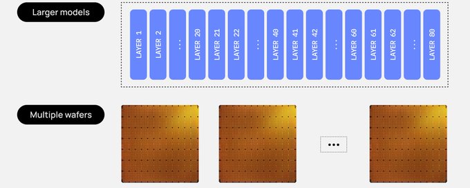 Written by Sarah Chieng, Head of DevX (@MilksAndMatcha) One of the most frequently asked questions we get is how we deploy large models on Cerebras wafer-scale chips. A single Cerebras WSE-3T wafer has 44 GB of on-chip memory, and trillion-parameter frontier models need terabytes for their weights alone. In this post, we’ll explain how we split a large frontier model across multiple WSE-3T wafers, to run multi-trillion parameter models at 1000-2000+ tokens per second. We’ll use the open source model Kimi K3, with ~3 trillion parameters, as an illustrative example. By the end, you'll understand: - How we fit the full model into on-chip memory - How we map the model across multiple chips - How we handle a high # of concurrent requests ## Breaking it down with Kimi K3 Kimi K3 is an open source, 3T parameter model with 69 linear-attention layers and 24 dense layers. 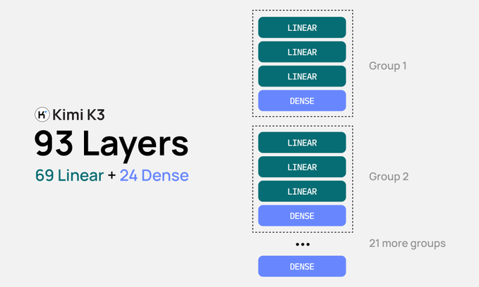 It scores an impressive 88.3% on Terminal-Bench 2.1 (vs. GPT-5.6 Sol's 88.8%) and 91.2% on BrowseComp (vs. GPT-5.6 Sol's 90.4%). These results demonstrate frontier-level coding and agentic capabilities, even outperforming leading proprietary models on some benchmarks. Read more about Kimi K3 here. 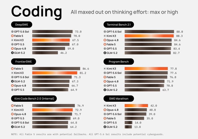 For this illustrative example, we use: - A 256k assumed average request size - 4-bit weight quantization (like the Hugging Face implementation) - An 8-bit KV cache ## #1: Size of Each layer To calculate the total number of Cerebras WSE-3T wafers we need to support Kimi K3, let’s first calculate the size of each model layer. Kimi K3 has 3 trillion parameters. If all 3T parameters are stored at 4 bits each, the raw parameter payload is: 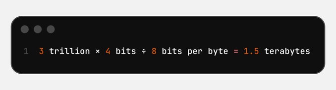 Dividing that payload by 93 layers then gives: 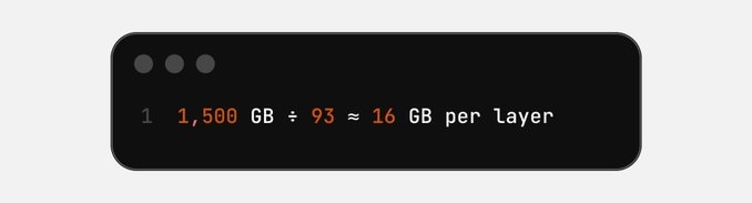 ## #2: Number of Wafers Now that we know each layer needs about 16 GB, we can figure out how many layers fit on each 44 GB wafer. The answer depends on the layer type: - Dense layers need additional room for a KV cache, because each dense (full-attention) layer stores the keys and values for every token in every active request. So, we place one dense layer per wafer and leave the remaining SRAM for its KV cache. - Linear-attention layers do not require additional room for a KV cache. Instead of storing keys and values for every token, a linear-attention layer keeps a small, fixed-size state per request, regardless of context length. That leaves room for two linear layers per wafer (2 × 16 GB = 32 GB). 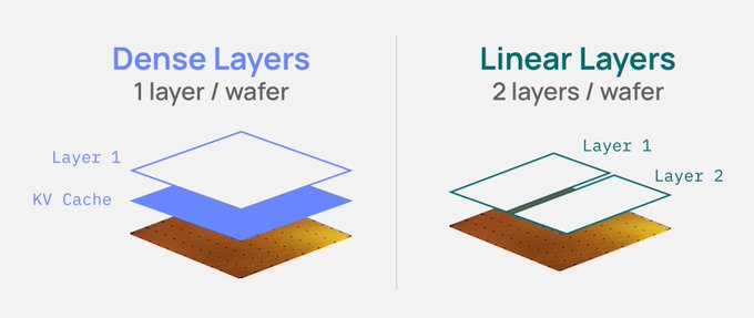 Therefore, with Kimi K3’s 69 linear layers and 24 dense layers, we get: 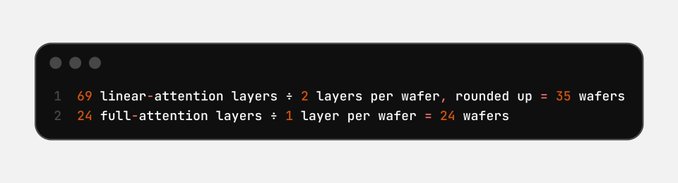 This gives us a total wafer count of 35 + 24 = 59 wafers. ## #3: Connecting the wafers together Cerebras executes models in a pipeline. After the Cerebras compiler maps the model layers across regions of wafers, the runtime maps the path for tokens to flow between wafers. For ultrafast latency, only activations need to be passed between the wafers, and this can be done via RDMA over Ethernet. This is roughly 2 microseconds per hop. 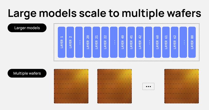 It’s important to emphasize that because each Cerebras wafer has 44 GB of on-chip SRAM and each layer is only 16 GB, we are typically able to fit entire layers of the model directly on the chip. This means that in most cases, the model weights never have to move, and layers don’t need to be split across wafers. Only activations cross from one wafer to the next. ## #4: How we serve 1 request Now that we have our wafers connected together and the model laid out, we can think of each wafer as one stage in an assembly line: the model’s weights for each stage stay in place, and the request’s intermediate results move through the layer stages. For example, Wafer 1 runs model layers 1–2 and sends its activations to wafer 2. Wafer 2 runs layers 3–4 and passes its results to Wafer 3, and so on until the last wafer produces the next token. 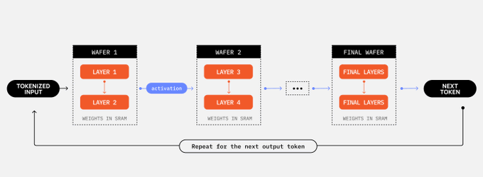 ## #5: How we serve many requests This raises a common misconception. If a token has to travel through each wafer in order, doesn’t each wafer sit idle while it waits for its turn? In effect, wouldn't the system be running at a batch size of one? No! If we only sent one request down the line at a time and waited for it to complete before starting the next request, this would be an inefficient use of the pipeline. Instead, we keep the entire pipeline full with different requests. Because the model is split into pipeline stages already, each stage can work on a different request at the same time. While stage 3 processes a token for request A, stage 2 processes one for request B, and stage 1 one for request C. In our example, each stage is a layer. In production, Cerebras uses much finer-grained stages, and many more of them. <video controls preload="metadata" poster="/doc/8703/image/img_98ec9404af3b.jpg" src="/videos/1679.mp4"></video> Each stage can also process a micro-batch, a small group of requests, rather than a single request. So the number of requests in flight is roughly the number of stages times the micro-batch size. <video controls preload="metadata" poster="/doc/8703/image/img_c17695e0fb8d.jpg" src="/videos/1680.mp4"></video> To understand the tradeoff, smaller micro-batches make each request even faster, while larger micro-batches increase total throughput. ## #6: How many requests can we serve? The amount of on-chip memory allocated to KV cache determines the maximum number of concurrent requests. Every request in flight needs its own KV cache on each dense-layer wafer, so the size of on-chip memory sets the ceiling on concurrent requests. As explained above, we only need to calculate KV cache requirements for dense layers. For each 44 GB wafer that already has one dense layer, we can calculate the remaining space for the KV cache with Total wafer storage - size of one dense layer. In this case:  Calculating the # of Concurrent Requests To find the number of concurrent requests supported for any particular model mapping, we first calculate how much cache a single 256k request takes up: 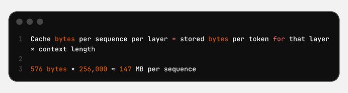 To then calculate the total number of concurrent requests this configuration would support, we divide: 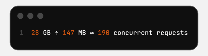 The total number of concurrent requests represents the number of simultaneous requests moving through the pipeline at any point in time. Unlike a GPU batch, those requests don’t wait for one another to finish, they stream through the pipeline continuously. Of course, neither concurrency nor batch size tells you exactly how efficiently an inference system performs. When evaluating the throughput of an inference system, the more meaningful metric is total token throughput per unit of power (e.g. tokens per second per megawatt), when measured at the same output generation speed. # How this scales beyond 3T parameters The same approach extends to larger models: calculate the memory needed for weights and request state, distribute the model across wafers, and connect them into a pipeline. Each additional wafer contributes compute and on-chip memory, allowing us to accommodate models that exceed the capacity of any single chip. Thanks for learning with us! Interested in deploying a model on Cerebras or building with our inference cloud? - Get started with our free API: cloud.cerebras.ai - Reach out to our sales team: sales@cerebras.ai - Read more articles at cerebras.ai - Read the original article here. Designs by @halleychangg. Thanks to Atharva Talpade, Zhenwei Gao, Angela Yeung, Jessica Liu, Joyce Er, Emma Call, and Rohan Guptafor their review and feedback. ## 相关链接 - [Cerebras](https://x.com/cerebras) - [@cerebras](https://x.com/cerebras) - [82K](https://x.com/cerebras/status/2113315017714246003/analytics) - [@MilksAndMatcha](https://x.com/@MilksAndMatcha) - [WSE-3T](https://www.cerebras.ai/chip) - [an impressive 88.3% on Terminal-Bench 2.1](https://www.kimi.com/en/blog/kimi-k3) - [Read more about Kimi K3 here](https://modal.com/blog/trillion-tokens-trillion-parameters) - [Hugging Face implementation](https://huggingface.co/moonshotai/Kimi-K3) - [69 linear layers and 24 dense layers](https://huggingface.co/moonshotai/Kimi-K3#2-model-summary) - [cloud.cerebras.ai](http://cloud.cerebras.ai/) - [sales@cerebras.ai](mailto:sales@cerebras.ai) - [cerebras.ai](https://www.cerebras.ai/blog) - [here](https://www.cerebras.ai/blog/how-we-deploy-trillion-parameter-frontier-models-on-cerebras) - [@halleychangg](https://x.com/@halleychangg) - [Upgrade to Plus](https://x.com/i/premium_sign_up) - [1:02 AM · Oct 23, 2026](https://x.com/cerebras/status/2113315017714246003) - [82.9K Views](https://x.com/cerebras/status/2113315017714246003/analytics) - [View quotes](https://x.com/cerebras/status/2113315017714246003/quotes) --- *导出时间: 2026/10/23 16:58:36* --- ## 中文翻译 # 我们如何在 Cerebras 上部署万亿参数前沿模型 **作者**: Cerebras **日期**: 2026-10-22T17:02:18.000Z **来源**: [https://x.com/cerebras/status/2113315017714246003](https://x.com/cerebras/status/2113315017714246003) **阅读**: 82947 **点赞**: 502 **转发**: 73 **回复**: 24 ---  作者:Sarah Chieng,DevX 负责人 (@MilksAndMatcha) 我们最常被问到的问题之一是:我们如何在 Cerebras 晶圆级芯片上部署大模型。单颗 Cerebras WSE-3T 晶圆拥有 44 GB 片上内存,而万亿参数的前沿模型仅权重就需要数 TB 的存储空间。 在这篇文章中,我们将解释如何将一个大型前沿模型拆分到多颗 WSE-3T 晶圆上,从而以每秒 1000-2000+ token 的速度运行数万亿参数的模型。 我们将使用开源模型 Kimi K3(约 3 万亿参数)作为示例。 读完本文,你将了解: - 我们如何将完整模型装进片上内存 - 我们如何将模型映射到多颗芯片上 - 我们如何处理大量并发请求 ## 以 Kimi K3 为例进行拆解 Kimi K3 是一个开源的 3 万亿参数模型,包含 69 层线性注意力层和 24 层稠密层。  它在 Terminal-Bench 2.1 上取得了令人瞩目的 88.3%(对比 GPT-5.6 Sol 的 88.8%),在 BrowseComp 上取得了 91.2%(对比 GPT-5.6 Sol 的 90.4%)。这些结果表明其具备前沿水平的编码和智能体能力,甚至在部分基准测试中超越了领先的专有模型。点击这里了解更多关于 Kimi K3 的信息。  在本示例中,我们使用: - 假设的平均请求大小为 256k - 4 位权重量化(类似于 Hugging Face 的实现方式) - 8 位 KV 缓存 ## #1:每层的大小 为了计算支持 Kimi K3 所需的 Cerebras WSE-3T 晶圆总数,我们先来计算模型每一层的大小。 Kimi K3 拥有 3 万亿参数。如果所有 3T 参数都以每位 4 比特存储,原始参数负载为:  将该负载除以 93 层,得到:  ## #2:晶圆数量 现在我们知道每层大约需要 16 GB,就可以算出每颗 44 GB 的晶圆上能放多少层。答案取决于层的类型: - 稠密层需要额外的空间存放 KV 缓存,因为每个稠密(全注意力)层都要为每个活跃请求中的每个 token 存储键和值。因此,我们在每颗晶圆上放置一个稠密层,并将剩余的 SRAM 留作其 KV 缓存。 - 线性注意力层不需要额外的 KV 缓存空间。线性注意力层无需为每个 token 存储键和值,而是为每个请求保留一个小的、固定大小的状态,与上下文长度无关。这样每颗晶圆可以容纳两个线性层(2 × 16 GB = 32 GB)。  因此,对于 Kimi K3 的 69 个线性层和 24 个稠密层,我们得到:  晶圆总数为 35 + 24 = 59 颗。 ## #3:将晶圆连接起来 Cerebras 以流水线方式执行模型。Cerebras 编译器将模型各层映射到晶圆的各个区域后,运行时会规划 token 在晶圆之间流动的路径。为实现超低延迟,晶圆之间只需传递激活值,这可以通过基于以太网的 RDMA 完成。每一跳大约耗时 2 微秒。  需要强调的是,由于每颗 Cerebras 晶圆拥有 44 GB 的片上 SRAM,而每层只有 16 GB,我们通常能够将模型的整个层直接装在芯片上。 这意味着在大多数情况下,模型权重完全不需要移动,层也不需要跨晶圆拆分。只有激活值会从一颗晶圆传递到下一颗。 ## #4:我们如何服务一个请求 既然晶圆已经连接起来、模型也已布局完毕,我们可以把每颗晶圆看作流水线上的一道工序:模型各阶段的权重保持原位,而请求的中间结果则在各层工序之间流转。 例如,晶圆 1 运行模型第 1-2 层,并将其激活值发送给晶圆 2。晶圆 2 运行第 3-4 层,并将结果传递给晶圆 3,依此类推,直到最后一颗晶圆生成下一个 token。  ## #5:我们如何服务多个请求 这引出了一个常见的误解。如果一个 token 必须依次经过每颗晶圆,那么每颗晶圆在等待轮到自己时岂不是处于空闲状态?实际上,系统岂不是以批大小为 1 在运行? 不是的!如果我们一次只发送一个请求进入流水线,并等它完成后再开始下一个请求,这会是对流水线的低效利用。相反,我们让整个流水线始终充满不同的请求。由于模型已经被拆分为流水线阶段,每个阶段可以同时处理不同的请求。 当第 3 阶段处理请求 A 的一个 token 时,第 2 阶段处理请求 B 的,第 1 阶段处理请求 C 的。在我们的示例中,每个阶段是一层。而在生产环境中,Cerebras 使用的是粒度更细、数量更多的阶段。 <video controls preload="metadata" poster="/doc/8703/image/img_98ec9404af3b.jpg" src="/videos/1679.mp4"></video> 每个阶段还可以处理一个微批次,即一小批请求,而不是单个请求。因此,同时在途的请求数量大约等于阶段数乘以微批次大小。 <video controls preload="metadata" poster="/doc/8703/image/img_c17695e0fb8d.jpg" src="/videos/1680.mp4"></video> 这里存在一个权衡:更小的微批次能让每个请求更快,而更大的微批次则能提高总吞吐量。 ## #6:我们能服务多少个请求? 分配给 KV 缓存的片上内存容量决定了并发请求的最大数量。每个在途请求在每个稠密层晶圆上都需要自己的 KV 缓存,因此片上内存的大小为并发请求的数量设定了上限。如上所述,我们只需计算稠密层的 KV 缓存需求。 对于每颗已承载一个稠密层的 44 GB 晶圆,我们可以用以下公式计算 KV 缓存的剩余空间: 晶圆总存储 - 一个稠密层的大小。在本例中:  计算并发请求数量 要找出某个特定模型映射方案所支持的并发请求数量,我们先计算一个 256k 请求占用多少缓存:  然后用除法计算该配置支持的并发请求总数:  并发请求总数表示在任意时刻同时在流水线中流动的请求数量。与 GPU 批处理不同,这些请求不需要互相等待完成,而是持续不断地流经流水线。 当然,无论是并发数还是批大小,都不能准确衡量推理系统的运行效率。在评估推理系统的吞吐量时,更有意义的指标是在相同输出生成速度下,单位功耗的总 token 吞吐量(例如每兆瓦每秒生成的 token 数)。 # 如何扩展到超过 3T 参数 同样的方法可以推广到更大的模型:计算权重和请求状态所需的内存,将模型分布到多颗晶圆上,并将它们连接成流水线。每增加一颗晶圆就带来额外的算力和片上内存,使我们能够支持超出单颗芯片容量的模型。 感谢与我们一同学习!有兴趣在 Cerebras 上部署模型或使用我们的推理云进行开发吗? - 免费使用我们的 API 入门:cloud.cerebras.ai - 联系我们的销售团队:sales@cerebras.ai - 在 cerebras.ai 阅读更多文章 - 点击此处阅读原文。 设计:@halleychangg。感谢 Atharva Talpade、Zhenwei Gao、Angela Yeung、Jessica Liu、Joyce Er、Emma Call 和 Rohan Gupta 的审阅与反馈。 ## 相关链接 - [Cerebras](https://x.com/cerebras) - [@cerebras](https://x.com/cerebras) - [82K](https://x.com/cerebras/status/2113315017714246003/analytics) - [@MilksAndMatcha](https://x.com/@MilksAndMatcha) - [WSE-3T](https://www.cerebras.ai/chip) - [在 Terminal-Bench 2.1 上取得令人瞩目的 88.3%](https://www.kimi.com/en/blog/kimi-k3) - [点击这里了解更多关于 Kimi K3 的信息](https://modal.com/blog/trillion-tokens-trillion-parameters) - [Hugging Face 实现](https://huggingface.co/moonshotai/Kimi-K3) - [69 个线性层和 24 个稠密层](https://huggingface.co/moonshotai/Kimi-K3#2-model-summary) - [cloud.cerebras.ai](http://cloud.cerebras.ai/) - [sales@cerebras.ai](mailto:sales@cerebras.ai) - [cerebras.ai](https://www.cerebras.ai/blog) - [此处](https://www.cerebras.ai/blog/how-we-deploy-trillion-parameter-frontier-models-on-cerebras) - [@halleychangg](https://x.com/@halleychangg) - [升级到 Plus](https://x.com/i/premium_sign_up) - [2026年10月23日 凌晨1:02](https://x.com/cerebras/status/2113315017714246003) - [8.29万次浏览](https://x.com/cerebras/status/2113315017714246003/analytics) - [查看引用](https://x.com/cerebras/status/2113315017714246003/quotes) --- *导出时间: 2026/10/23 16:58:36*
A AI 工程师面试:大厂反复考的 25 道通用题 文章总结了 AI 工程师面试中各科技大厂(OpenAI、Meta、DeepSeek、Anthropic 等)反复考察的高频题目,覆盖三大模块:LLM 内部原理(attention、KV cache、RoPE、MoE、scaling laws、解码策略等)、推理部署与 GPU 性能(continuous batching、PagedAttention、量化、并行策略、显存估算、延迟指标等),以及 RAG、Agent、微调、评测、安全、多模态、系统设计等方向。作者指出各家面试题高度重合,建议优先刷这些通用题以获得最高性价比。 技术 › LLM 山景城小路 2026-10-07 面试LLMTransformerKV cache推理部署量化并行策略scaling lawsAI工程师大模型
显 显存就这么多,怎么把字吐得更快?——从 MoE、KV Cache 到 DFlash 的本地部署全景拆解 文章从一张16GB显卡出发,系统拆解大模型本地部署的显存与速度权衡。首先澄清运行显存不只包含模型权重,还有KV Cache、运行时工作区和草稿模型开销;解释MoE与量化对容量和计算的不同影响,区分总参数与激活参数;分析CPU/GPU卸载的代价;介绍KV Cache与混合注意力如何影响上下文长度;区分Prefill与Decode两个阶段的速度特征;最后详解投机解码、MTP与DFlash/DFlash2的加速原理及实测收益。强调各优化手段需配合使用,预算刚好装满并不代表能稳定运行。 技术 › LLM huangserva 2026-09-14 本地部署MoEKV Cache量化投机解码DFlash显存优化推理加速大模型
K KV Cache Engineering for LLM Serving, clearly explained 文章系统讲解了LLM推理中KV缓存的工程优化。KV缓存随序列长度增长,Llama 3.1 70B单条128K序列的BF16缓存约需40GB,成为GPU内存和注意力计算的双重瓶颈。作者将12种优化技术按减少的对象分类:GQA/MQA减少KV头数量,跨层注意力减少缓存层数,滑动窗口与淘汰减少保留token数,MLA减少表示宽度,量化减少字节数,混合循环层用固定状态替代增长缓存,分页与前缀复用减少分配浪费。文章配有可运行代码示例,并分析各技术的适用场景与权衡。 技术 › LLM Avi Chawla 2026-09-06 KV CacheLLM推理GQAMQA量化GPU内存注意力机制模型优化推理加速Llama
1 12G显存部署125B Qwen3.8-Flash-Next 全攻略 本文介绍如何在12GB显存上部署125B参数的Qwen3.8-Flash-Next模型。核心是Strata技术让GPU、CPU、RAM和SSD协同工作:常用专家留GPU,其余放RAM,CPU处理cache miss。RTX 5070 12GB + 64GB RAM在Q2_0量化下短对话可达94 tok/s。文章还讲解了量化选择策略——显存占用相同时速度可差1.72倍,关键在于专家命中率。作者全程使用蚂蚁的Ling-3.1-flash Agent自动完成从检查机器、选权重、下载安装到排错验收的完整部署流程,跑通了一套用Agent自动部署本地模型的可复用方法。 技术 › LLM 实践哥 Li 2026-10-08 QwenStrata本地部署量化MoEAgentLing-3.1-flash显存优化推理加速12GB显卡
D Disaggregated Inference From The Ground Up 本文由 Cerebras 撰写,从基础原理讲解推理系统中的分离式推理技术。文章先介绍加速器的构成(计算单元与存储),并引入算术强度概念,通过矩阵加法与矩阵乘法的实例说明数据搬运与计算的关系。随后分析 LLM 推理的两个阶段:prefill(处理整个 prompt,计算密集型)与 decode(逐 token 生成,受限于内存带宽),解释二者对硬件需求的不同。Cerebras 提出异构分离式推理,将不同类型芯片分配给不同推理阶段,在相同硬件数量下将吞吐量提升 5 倍且不损失单用户生成速度。 技术 › LLM Cerebras 2026-10-02 Cerebras推理disaggregation算术强度prefilldecode加速器GPUKV cache硬件
W We built a 20x faster Grok bot Cerebras 团队测试了主流 AI 个人助理完成订餐任务的表现,发现现有助理耗时过长(如 Grok Bot 需 7 分 40 秒)。团队使用 Qwen 3.8 27B 模型运行在 Cerebras 硬件上,以 Pi 作为 Agent Harness,通过三项优化将任务压缩至 22 秒:1) 并行执行独立的检查操作;2) 借助 Cerebras 快速推理加速模型调用;3) 将探索网站的经验固化为 Skill 复用,减少 80% 以上的工具调用。文章展示了 Harness Engineering、快速推理和经验沉淀对 Agent 效率的巨大提升潜力。 技术 › Agent Cerebras (Sarah Chieng, @0xSero) 2026-09-26 CerebrasAgentGrokHarness EngineeringSkillQwenLLM推理加速OpenClaw性能优化
L LLM Inference Handbook 精读:Prefill、Decode、KV Cache,与一切皆权衡的推理工程 本文深度解读 Modular 公司开源维护的《LLM Inference Handbook》,系统梳理 LLM 推理工程的知识体系。文章提炼三大核心框架:prefill(算力受限)与 decode(带宽受限)的两阶段二分法;KV cache 作为系统中心约束的地位,围绕它的 PagedAttention、prefix caching、PD 分离等技术网络;以及“一切皆 trade-off,唯一方法论是 benchmark”的工程哲学。内容还涵盖 continuous batching、speculative decoding、GPU 内存金字塔、FlashAttention、量化与蒸馏三部曲、Agent 生态与部署运维等主题,强调推理优化的本质是围绕有状态 KV cache 做内存管理与调度。 技术 › LLM meng shao 2026-09-22 LLM推理KV CachePrefillDecodeFlashAttention量化推理优化GPUBenchmarkPagedAttention
深 深读免费书「Inference Engineering」:Prefill 吃算力、Decode 吃带宽,讲透从 CUDA 到生产部署的推理优化 文章深度解读 Baseten 出版的免费工程书《Inference Engineering》,系统讲解如何把 AI 模型在生产环境中跑得快、省、稳。全书以三层推理栈(运行时、基础设施、工具层)为骨架,核心分析框架是瓶颈判断:prefill 算力受限、decode 带宽受限、图像视频生成算力受限。内容涵盖模型与硬件理解(算术强度、KV cache、选卡策略)、软件栈(vLLM/SGLang/TensorRT-LLM 三大引擎对比)、五大加速技术(量化、投机解码、缓存、并行、分离部署)及其交互关系,以及生产化部署的延迟全栈账本、故障处理与成本核算,强调约束换性能、技术按组合评估等基本原则。 技术 › LLM meng shao 2026-09-21 推理优化CUDA量化投机解码KV cachevLLMGPU生产部署读书笔记Inference Engineering
大 大开眼界:把 DeepSeek V4.1 Flash 的 Causal Encoder-Decoder 思路移植到 Qwen3-8B 文章介绍了一项实验:研究者将 DeepSeek V4.1 Flash 的 Causal Encoder-Decoder 机制移植到现有 Qwen3-8B 上,不修改原模型权重,仅外挂一个小模型近似后半层 KV Cache,使 Prefill 时间缩短近一半且输出一致。作者分析了这对本地模型部署(尤其 DGX Spark)的重大意义:长上下文首 token 等待明显降低,KV Cache 内存占用减少,Coding Agent、Computer Use Agent 等本地工作负载体感大幅提升。文章同时指出结果尚需在更多任务上验证,但认为已有模型可通过轻量近似层获得架构级推理升级。 技术 › LLM Wei (@wei_wang) 2026-09-13 DeepSeekQwen3-8BPrefill优化KV Cache本地模型DGX Spark推理加速Agent架构创新Encoder-Decoder
图 图解大语言模型部署 本文系统讲解大语言模型自部署的核心指标与实践要点,覆盖延迟类指标(TTFT、TPOT/ITL、P95/P99)、吞吐类指标(TPS、QPS、连续批处理)、资源类指标(显存与KV cache计算、量化精度)、服务质量(错误率、探针、可用性)以及成本核算(cost per token、TCO)。作者以 Ling-3.0-Flash MoE 模型在 DGX Spark 上的真实实测为例,将抽象指标落地为具体数字,帮助读者选对硬件配置、排查吞吐瓶颈与OOM问题、评估自建与API的划算临界点。 技术 › LLM WquGuru 2026-08-29 LLM模型部署推理优化显存KV cacheTTFT吞吐量量化vLLM成本核算
L LLM 中的 KV Cache、Prefix Cache、Prompt Cache 与 Semantic Cache 详解 文章系统讲解了 LLM 推理中四层常被混淆的缓存机制:KV cache 存储单次请求的注意力张量;Prefix caching 在服务端以 token ID 哈希链为键复用这些张量;Prompt caching 是服务商对该查找的计费版本;Semantic cache 则以嵌入向量的余弦相似度为键存储完整响应。前三层为精确匹配、不影响正确性,未命中只损失延迟和费用;第四层为模糊匹配,可能返回错误答案。文章基于 transformers v5 提供可运行代码示例,涵盖缓存增长、内存带宽瓶颈、GQA/MLA/量化等优化手段,以及阻碍缓存复用的五类常见问题。 技术 › LLM Avi Chawla 2026-08-28 KV CachePrefix CachingPrompt CachingSemantic CacheLLM 推理transformers注意力机制缓存优化内存带宽量化
B BestBlogs 早报 · 08-14|DeepSeek Harness 智能体,GPT-5.6 Sol 压缩推理等待,多智能体实验暴露协作失灵 本期早报聚焦智能体系统的三大核心问题:架构、算力与协作机制。DeepSeek Harness 提供插件化 Agent Harness,将模型、工具等能力拆分为可替换组件;Cerebras 与 OpenAI 推出 GPT-5.6 Sol Ultrafast,通过专用硬件实现高速推理;Anthropic 的多智能体实验揭示了协作中的冲突、从众与信任问题。此外,速览部分涵盖 Gemini 3.7 Flash 发布、Agent 评测与轨迹复盘、ICML 论文复现经验、Claude Tag 更新及小红书开源 TTS 模型。 技术 › LLM ginobefun 2026-08-14 智能体DeepSeek HarnessGPT-5.6多智能体推理加速插件化协作机制AnthropicCerebras早报