# On SFT, RL, and on-policy distillation
**作者**: will brown
**日期**: 2026-05-01T02:23:07.000Z
**来源**: [https://x.com/willccbb/status/2050038277454143918](https://x.com/willccbb/status/2050038277454143918)
---
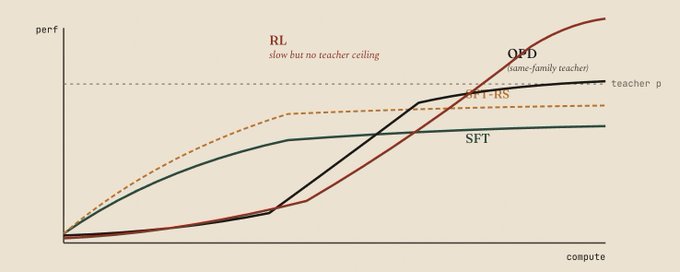
Why the SFT-RL pipeline works, where on-policy distillation fits, and how self-distillation goes wrong.
Authors: Will Brown & Claude Opus 4.7
April 30, 2026
[Editor's Note: Arguments are mine, writing is Claude's. This is partially an experiment in trying to get Claude to help speed-write and structure technical research blogs, drafted initially as artifacts and refined via "debate". I have too many blog ideas that I never get around to writing up, but the models finally feel good enough to help out with this (hopefully -- let me know what you think).]
## §1 — The standard pipeline and the compounding argument
Most post-training pipelines are some version of "SFT first, then RL" — pre-train, supervised-finetune to get a baseline, then run RL once SFT data dries up or stops moving the needle. People usually treat this ordering as a convention, but there's a real argument for it that's worth being explicit about. The argument is about which sampling distribution your method gets to compound with, and where the resulting performance ceiling sits.
When I say SFT in this post I mean teacher SFT: training on completions produced by some teacher model. (Plain instruction-tuning on human-curated data is the same shape, with humans as the teacher.) The defining property is that the sampling distribution is fixed at dataset-construction time. As the model improves during training, the data does not. Once the student gets close to the teacher's distribution, more SFT mostly memorizes — the marginal example is no longer informative. SFT's ceiling is roughly the teacher's.
RL is the opposite. The student samples its own rollouts, the gradient updates the policy, and the next batch is sampled from the improved policy. Improvements compound back into the sampling distribution. The ceiling isn't determined by the data — it's determined by whatever the verifier can grade.
This produces a tipping point. When current performance is far below the teacher and teacher data is cheap, SFT bits are extremely cheap-per-improvement — you're learning capabilities you don't have, from a source that does. As current performance approaches the teacher, marginal SFT examples get less informative, and the student's own rollouts start producing genuinely new strategies via lucky exploration that an RL gradient can extract. Past the tipping point, rollout compute is better spent on RL than on more SFT.
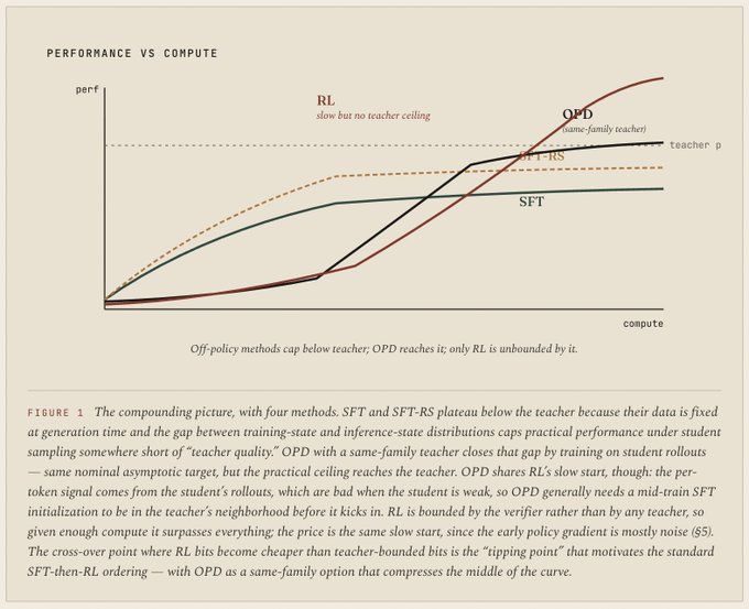
Rejection-sampled SFT (SFT-RS, sometimes RFT — sample from the teacher or the student, filter for correctness, train on the survivors) is strictly better than vanilla teacher SFT in expectation, but it doesn't fix the compounding problem. The sampling distribution is still pinned to whatever you're filtering. Once your filter saturates — everything correct is included, everything wrong is discarded — you've hit the same ceiling. SFT-RS shifts the curve up, but it doesn't change its shape.
None of this is new, but it's worth saying clearly because everything else in this post is about how to push past that ceiling, and the available moves depend on what you have access to.
## §2 — Same-family vs. different-family teachers
"Doing SFT" involves choosing a teacher, and the teacher's relationship to your student is a major axis of efficiency that doesn't get enough attention.
Same-family teacher means tokenizer-matched and recipe-matched: same vocabulary, same general training pipeline, ideally the same base model at different scales. Qwen3-32B teaching Qwen3-8B-Base is the canonical example, originating in the Qwen3 technical report and revisited prominently in Thinking Machines' OPD post. The teacher's outputs sit in a distribution that's structurally close to what the student naturally produces. The SFT signal — for each token, "the teacher would have said this" — is mostly about the capability gap, not stylistic differences. Per-token logprobs from the teacher are directly comparable to the student's, because the vocabulary is shared and similar training recipes produce similar distributional shapes.
Different-family teacher means tokenizer mismatch, recipe mismatch, or both. Distilling a frontier closed model into an open base, or moving across model families. Two specific costs:
- Tokenizer mismatch means every teacher completion has to be re-tokenized in the student's vocabulary. You lose information at boundaries, and per-token logprobs no longer correspond to "the same prediction at the same position" between models. Soft-target distillation is essentially impossible without expensive workarounds.
- Recipe mismatch means the teacher's outputs carry stylistic and structural artifacts — how it formats lists, when it uses chain-of-thought, what register it speaks in — that are pipeline byproducts, not capabilities. The student has to absorb those alongside the actual content. A nontrivial fraction of the SFT bits go toward learning surface form rather than competence, and the resulting student often looks like a slightly worse version of the teacher's style without having internalized the teacher's reasoning.
Most cross-family distillation in practice loses something in the gap between "what the teacher knows" and "what the student can absorb without learning the teacher's pipeline." Same-family SFT is much more efficient per unit of capability transferred, even if you can't always afford to limit yourself to it.
This matters because the next move on the algorithm tree — on-policy distillation — is essentially only available in the same-family setting, and that constraint shapes the rest of this post.
## §3 — On-policy distillation as the same-family upgrade
On-policy distillation (OPD, as in Lu et al. 2025 and the Qwen3 technical report before it) is the obvious move once you've laid out the previous two sections. The student samples its own rollouts — so you get RL's compounding in the sampling distribution — but each token in the rollout is graded by the teacher via per-token reverse KL:
The advantage at each token is "how much the teacher prefers this token relative to the student." Dense, on-policy, reverse-KL. The reported numbers are striking — roughly 9–30× less compute than RL on AIME-style benchmarks, with the gap widening when teacher logprob calls can be parallelized.
This raises a question that figure 1 implicitly answers: why does OPD's practical ceiling sit above SFT-RS's, when both target the same teacher? Cheaper sampling is part of it — the teacher only forward-passes over student tokens, which is essentially prefill, and prefill is much cheaper per FLOP than generation. But that mostly buys faster convergence, not a higher ceiling. The deeper reason is on-policy state coverage. SFT and SFT-RS train under the teacher's state distribution but evaluate the student under its own; the exposure-bias gap that opens up over long rollouts caps off-policy practical performance somewhere short of "teacher quality" on the actual evaluation distribution. OPD trains on student rollouts, so the gap doesn't open. Same nominal asymptotic target, different practical ceiling.
The catch is that OPD requires a same-family teacher, and the dependence is harder than people often acknowledge. You need tokenizer match just to compute the loss — the per-token KL is between teacher and student distributions over the same token positions. You also need at least approximate recipe match, because the per-token signal needs to actually be informative on the things you care about. If the teacher and student were trained with very different recipes, the reverse-KL gradient is dominated by "the teacher would have phrased this differently" rather than "the teacher would have reasoned differently here."
So OPD is the "best of both worlds" corner only when you have a same-family teacher available. When you do, it tends to dominate at moderate compute budgets — do mid-train SFT to get into the teacher's rough neighborhood, then OPD instead of RL to approach the teacher's level efficiently (you get to explore with a smaller model, and prefill is cheap). The ceiling is a different question. OPD targets the teacher's distribution by construction, so in the limit it's bounded by the teacher; RL's ceiling is bounded by the verifier, which can be much higher. So the framing isn't "OPD beats RL," it's "OPD gets you to the teacher's level much faster than RL would, and most of the time that's where you wanted to be anyway." When you don't have a same-family teacher, you fall back to either cross-family SFT (eat the recipe-mismatch tax) or RL (eat the sparsity tax) — or, more recently and speculatively, to self-distillation.
## §4 — When you don't have a same-family teacher
The natural response to "OPD is great if you have a same-family teacher" is "what if I don't?" Self-distillation tries to answer this by using the student itself as the teacher, with privileged information in the teacher's context that the student doesn't see at sampling time. Two instantiations have shipped recently; they share the same algorithmic shape and differ only in what privileged info goes to the teacher.
SDFT (Shenfeld et al. 2026) conditions the teacher on an expert demonstration — a worked example, possibly for a different task. Student samples a trajectory without the demonstration in context; teacher computes per-token logprobs over the trajectory while seeing the demonstration; student updates toward teacher via reverse KL. Fully on-policy. The demonstration provides distributional pull without leaking the answer, and the paper makes the assumption underpinning this explicit (more on that in §8).
OPSD (Zhao et al. 2026) conditions the teacher on the ground-truth answer instead. Same setup otherwise. The teacher knows where the trajectory is supposed to end up; the student doesn't. This produces a much sharper distributional shift in the teacher than a demonstration does.
In both cases tokenizer match is automatic (same model). Recipe match is automatic (same model). What you trade for that is that the privileged-info conditioning shifts the teacher's distribution — modestly for SDFT, more aggressively for OPSD — away from the student's natural distribution.
Both sit at exactly the same dial settings as OPD. The only difference is the choice of teacher. That difference turns out to be where the failure mode lives.
## §5 — The geometry of gradients
To see why, it's worth working through what each method's gradient actually looks like in parameter space. The shapes are different in instructive ways.
RL: sparse, but saved by destructive interference
The standard complaint about RL is one bit per episode — a binary "you got it right" spread across thousands of tokens. The framing I find more useful: the apparent sparsity is what keeps RL's gradient updates honest.
In a GRPO-style step, every token in every rollout gets an advantage. Within a group, the advantages have approximately zero mean by construction (subtract the group baseline) and some variance. Each per-token advantage gets multiplied by the gradient of the log-probability of that token, producing a vector in parameter space. The total update is the average over the batch.
Most of those vectors are noise. Reward is sparse and broadcast-assigned; most tokens didn't actually contribute to whether the answer was right. Their advantages are nonzero only because they happened to share a trajectory with a reward, not because they were causally responsible for it. So the batch contains a swarm of small, mostly-random parameter-space vectors, with a small consistent bias along whichever dimensions actually correlate with reward ("think longer," "double-check arithmetic").
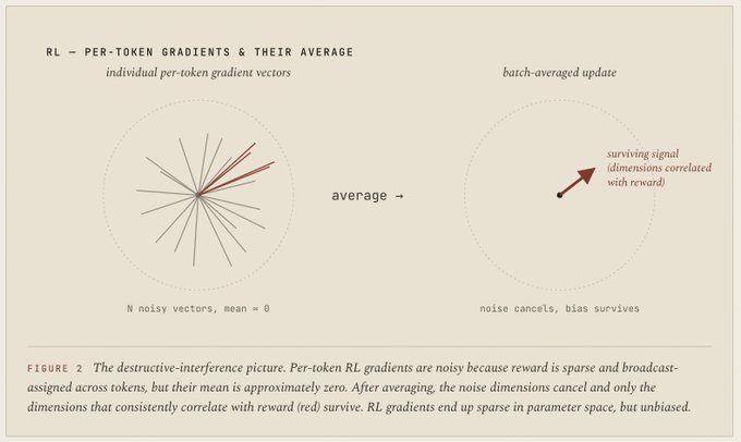
The reason large-batch, low-learning-rate RL is robust is not that each per-token gradient is informative — most aren't — but that the uninformative ones cancel. What survives the average is the small consistent component along the directions that actually correlate with reward. There's some empirical support for this: RL updates have been observed to be sparse in parameter space, modifying small subnetworks. That seems like the destructive-interference picture cashing out.
It also explains why RL feels "safe but slow." Each step moves the model a tiny amount in a direction you can trust. The sparsity isn't purely a bug; it's the price for an unbiased estimator.
SFT: dense, biased, but spread out
SFT does the opposite. Every token gets a one-hot label. The gradient density is enormous — one informative update per token, no broadcasting required.
But the SFT gradient distribution does not have zero mean. By construction, it's biased toward the data distribution. There's no analog of advantages cancelling. Constructive interference, not destructive.
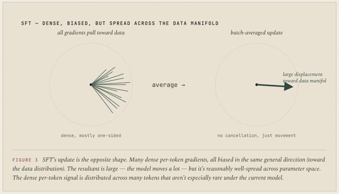
So why doesn't SFT blow up? Two reasons. First, the data distribution is itself diverse: the bias points in many slightly different directions across many examples, so you get a soft principal-components decomposition where the model drifts toward the data manifold as a whole rather than any one example. Second, SFT is diffuse. Most of what an SFT step is doing is reinforcing things the model already half-knew. There aren't many tokens where the data is asking the model to put large mass on something it currently treats as near-zero probability.
This is why SFT is forgiving. The data can be a bit messy, the learning rate can be a bit off, and you mostly drift. The bias is real, but it's unconcentrated.
OPSD: dense, biased, and concentrated
OPSD's gradient has a different shape from either of the above, and the difference is instructive — it points at why pure self-distillation isn't quite the final answer.
Consider a long math rollout where the student gets the answer wrong because, somewhere in the chain of thought, it failed to make a key observation — pick the right substitution, notice a trick. Call that token (or short span) the pivot token. For the student, the probability of producing the pivot token might be very low — say 0.01. For the teacher, conditioned on the answer, the probability of that same pivot token is much higher — say 0.6, because once you know where the solution is going, the right substitution becomes obvious.
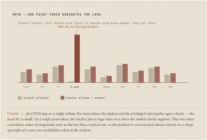
The per-token reverse KL between "student says 0.01" and "teacher says 0.6" is roughly log(0.6/0.01) ~= 4.1. For a typical token where both put around 0.3, the contribution is essentially zero. So one pivot token contributes on the order of a hundred times more to the loss than a typical one. The gradient is dominated by it.
What does that gradient do? It pushes the student's log-probability of the pivot token up sharply, given the prefix. The corresponding direction in parameter space is "make this rare token less rare in this context." Critically, this update is not being averaged against many other vectors pointing different directions. RL's saving grace was that noise vectors cancelled. SFT's saving grace was that bias was diffuse across many tokens that the student already supports. OPSD has neither. One concentrated tug, in one step, toward a region the model didn't previously believe in.
OPSD ships with per-token point-wise KL clipping — cap the per-vocabulary-entry divergence contribution at each position so that, in their words, "a small subset of stylistic tokens [doesn't] dominate the training signal." Without it, the paper reports performance collapse within ~100 steps. That's figure 4 cashing out. The fix works, and what it tells us is direct: the KL signal in self-with-hint distillation is concentrated enough that you have to budget it. The next move, then, is to look for a teacher whose KL is naturally diffuse, rather than relying on clipping to make a concentrated one tolerable.
## §6 — The sparse/dense × biased/unbiased family
The gradient analysis above places each method in a small taxonomy. The two main axes are sparse vs. dense (does each token get a signal, or just the trajectory) and biased vs. unbiased (does the expected gradient point in a fixed direction relative to the student, or only along the directions reward correlates with).
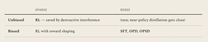
SFT, OPD, and OPSD all live in the "dense, biased" cell. They're distinguished by where the bias points (toward the data, toward a same-family teacher, toward self-with-hint) and, more importantly for the failure-mode analysis, by how that bias is distributed across tokens. That's the third axis — concentration:
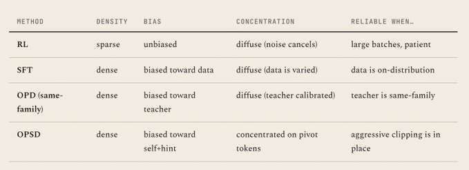
This is the punchline of the geometric analysis. RL is sparse but unbiased. SFT is dense and biased but diffuse. Same-family OPD inherits SFT's diffuseness because the teacher distribution is calibrated to the student's family. OPSD is the unique case where you get density, bias, and concentration at once — which is why it ships with explicit defenses (KL clipping, fixing the teacher to the initial policy) that the other methods don't need.
## §7 — An illustrative meta-algorithm
All four methods are special cases of a single token-level policy gradient:

with two scalar knobs and a teacher-policy choice:
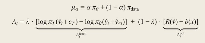
- α ∈ [0,1] — how on-policy the sampling distribution is.
- λ ∈ [0,1] — how much of the per-token advantage comes from a teacher KL versus a sequence-level outcome reward.
- π_T — the teacher policy: which model, conditioned on what context c_T.
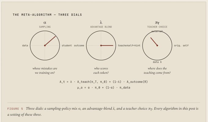
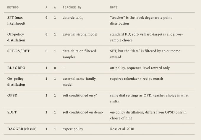
Once you fix α and λ, almost everything that matters — bias, concentration, stability — is a function of how π_T differs from π_θ at the per-token level on the student's rollouts. The interior of this space — α, λ ∈ (0,1), or mixed teacher choices — is mostly unexplored, and seems like where the next round of progress lives.
A few things drop out:
- SFT is "distillation from a degenerate teacher": letting π_T(y|x) = δ_{y_data}(y) recovers cross-entropy up to constants. The reason SFT is safe is not that this teacher is bad — it's that it's averaged across many varied examples, which makes the bias diffuse.
- RL is "no teacher": set λ=0 and the per-token signal collapses to broadcast outcome reward. The destructive-interference story follows from this.
- OPSD has identical dial settings to OPD: the only difference is π_T. That clarifies why it can match OPD when it works (same algorithm) and why it's where the failure mode is sharpest (most distributionally aggressive choice of teacher).
A caveat about what this factorization is for: it’s illustrative of the kind of algorithm conceptually aligned with the Pareto / SFT-RL phase-change picture — not a recommendation to mix sources at intermediate (α, λ). I’m not sure that’s even a useful algorithm. The clean corners (SFT, RL, OPD) are where the statistics work out without importance-sampling corrections, and they correspond to qualitatively different regimes that differ mostly in the KL budget β. The interesting axis of variation across them is β; interpolating α and λ is a tangent.
The practically-interesting structure looks more like “pick β, then find the best teacher for that β.” The meta-algorithm above makes the corners visible, but the actually hard problem is the inner one — and teacher optimization isn’t clean or cheap. It’s typically discrete (which model? which prompt? which hint?) and doesn’t decompose neatly into the gradient framing. The Pareto picture in §8 is where that question actually lives.
## §8 — Toward an optimal teacher
The geometry analysis turns the optimal-teacher question into an optimization problem. We want a teacher policy π_T that produces a large reward improvement on the student per step, subject to a hard KL constraint that keeps updates stable. In Lagrangian form:

This traces a Pareto curve as β varies. Different methods are different points on it.
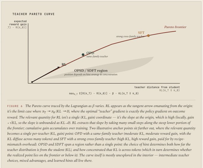
The SDFT paper's framing is worth engaging with directly here, because it offers a candidate route to the curve's interior that doesn't quite work for the reasons we want it to. The paper formalizes the ICL assumption — that a model conditioned on an expert demonstration approximates the optimal policy for the task — and conditions its analysis on the availability of such demonstrations. That assumption is doing a lot of work. Practically, this gives a similar ceiling (conceptually) to SFT and SFT-RS: you're only as good as the demonstrations, and you can't bootstrap beyond them.
We'd rather be in a world with curves more like RL, where the ceiling is only a function of our ability to verify, even if we can't always solve (without extremely expensive sampling). We can make weaker assumptions about the ability to verify (which we need anyway if we want to measure performance) plus mild regularity conditions on the distribution: that performance in accuracy degrades gracefully across the task distribution in a smooth latent space coupling task characteristics to the model's solve likelihood for a given checkpoint, and that updates should be net-positive-EV in distribution solve rate when sufficiently well-regularized — the high-batch-size, low-learning-rate, unbiased limit of, e.g., infinite-batch RL. This is what's needed for compounding gains where the only ceiling is the grader's performance, with the question being how to get there faster while retaining stability.
Policy gradient — at least within outcome-reward GAE — is roughly a minimum-variance unbiased estimator for the gradient of expected reward. The aim is to be able to turn a knob that trades bias for stable-yet-aggressive updates. OPD and SFT are two points on this curve, but both need a real teacher. Using a bigger smarter model improves the teacher but isn't directly workable for OPD without tokenizer match. There are cross-tokenizer methods, but ultimately we want something that lets us sweep teacher performance versus bias cleanly and cost-effectively.
Several plausible approaches target this objective at different levels of the stack:
- Per-task prompt optimization over the Lagrangian. Use something like GEPA over the Lagrangian objective on a per-task basis, with teacher sampling to estimate rewards. The optimizer searches the space of prompts (hints, conditioning) for the one that maximizes E[Δreward] − β·KL on the current student. This is a cheap inner loop that can produce a usable teacher without retraining anything.
- Distribution-level prompt optimization. Train a model to write good minimal hints when given a "bad" hint — whitebox RF access, the answer itself, a known-good demonstration. The training signal is the same Lagrangian, aggregated across the task distribution. The output is a hint-rewriter that turns large privileged-info hints into small ones that move the teacher distribution as little as possible while still improving reward.
- Self-prompt-optimization online RL. Treat hints as rollouts in a parallel environment that improves alongside the main policy via an RL objective, with loss components balanced adaptively (e.g., a smoothed minmax over reward-delta and KL terms). The hint-writer and student co-evolve.
- Train a hint-writing model directly with RL. Use correctness-delta × (1 − KL-delta) as the objective, scoped to a specific model / distribution / task / "in general" (the same way scopes work for judge-model training). The hint-writer is a separate artifact you can ship.
- Borrow from "expert RL + OPD." Some recent models (e.g. DeepSeek V4) layer a teacher signal on top of locally-optimal RL — an analog of the meta-algorithm with both a teacher KL and an outcome reward live simultaneously. The lessons from that line are directly relevant here.
What unifies these is that they all target the Lagrangian objective without requiring a fixed external teacher policy: the "teacher" is constructed (per task, per distribution, or online) to be locally optimal for the current student — high reward, low KL, surgical rather than broadcast.
In the limit, RL might still be optimal in the infinite-compute regime for the hardest heavy-tail problem distributions — the cases where any teacher distribution adds bias the student would've eventually corrected anyway. But it seems quite plausible that there's a nice meta-algorithm for interpolating more cleanly between distillation and RL: without needing a real teacher, and with compute-optimal learning at each point along the curve. Working that out is the open question I find most interesting in this space.
References
· Lu, K. & Thinking Machines Lab. On-Policy Distillation (2025).
· Zhao, S. et al. Self-Distilled Reasoner: On-Policy Self-Distillation for Large Language Models (OPSD, 2026).
· Shenfeld, I. et al. Self-Distillation Enables Continual Learning (2026).
· Agarwal, R. et al. On-Policy Distillation of Language Models: Learning from Self-Generated Mistakes (2023).
· Mukherjee, A. et al. Reinforcement Learning Finetunes Small Subnetworks in Large Language Models (2025).
· Qwen Team. Qwen3 Technical Report (2025).
· Ross, S. et al. A Reduction of Imitation Learning and Structured Prediction to No-Regret Online Learning (DAGGER, 2010).
## 相关链接
- [Pollux9437 reposted](https://x.com/Orange41324306)
- [will brown](https://x.com/willccbb)
- [@willccbb](https://x.com/willccbb)
- [46K](https://x.com/willccbb/status/2050038277454143918/analytics)
- [10:23 AM · May 1, 2026](https://x.com/willccbb/status/2050038277454143918)
- [46.1K Views](https://x.com/willccbb/status/2050038277454143918/analytics)
- [View quotes](https://x.com/willccbb/status/2050038277454143918/quotes)
---
*导出时间: 2026/5/1 14:40:54*
---
## 中文翻译
# 关于 SFT、RL 和在线策略蒸馏
**作者**: will brown
**日期**: 2026-05-01T02:23:07.000Z
**来源**: [https://x.com/willccbb/status/2050038277454143918](https://x.com/willccbb/status/2050038277454143918)
---

为什么 SFT-RL 流程有效,在线策略蒸馏处于什么位置,以及自蒸馏为何会出错。
作者:Will Brown & Claude Opus 4.7
2026 年 4 月 30 日
[编者注:观点属于我,写作由 Claude 完成。这部分是一次实验的尝试,旨在让 Claude 协助快速撰写和构建技术研究博客,最初以“artifacts”形式起草,并通过“辩论”进行优化。我有太多博客想法从未动手成文,但模型的感觉终于好到可以帮忙了(希望如此——请告诉我你的想法)。]
## §1 — 标准流程与复利论证
大多数后训练流程都是某种版本的“先 SFT,后 RL”——先预训练,再进行监督微调(Supervised-finetune)以获得基线,然后一旦 SFT 数据枯竭或不再能推动指标提升,就运行 RL。人们通常将这种顺序视为一种惯例,但实际上有一个强有力的理由支持这样做,这个理由值得明确指出。这个论点关乎你的方法能够与哪种采样分布产生复利效应,以及由此产生的性能天花板在哪里。
当我在本文中说 SFT 时,我指的是教师 SFT(teacher SFT):即基于某个教师模型生成的补全(completions)进行训练。(基于人工策划数据的普通指令调优也是同一性质,只是人类作为教师。)其定义属性是采样分布在数据集构建时是固定的。随着模型在训练过程中的改进,数据并不会改进。一旦学生接近了教师的分布,更多的 SFT 基本上就变成了死记硬背——边际样本不再提供信息。SFT 的天花板大致就是教师的天花板。
RL 则相反。学生采样自己的推演,梯度更新策略,下一批次从改进后的策略中采样。改进反馈回采样分布,形成复利。天花板不是由数据决定的——而是由验证器能够评分的内容决定的。
这产生了一个临界点。当当前性能远低于教师且教师数据廉价时,SFT 的比特具有极高的性价比——你正在从一个拥有能力的来源学习你尚未具备的能力。随着当前性能接近教师,边际 SFT 样本的信息量降低,学生自己的推演开始通过幸运的探索产生真正的新策略,而 RL 梯度可以提取这些策略。越过临界点后,与其将推演算力花费在更多 SFT 上,不如花费在 RL 上。

基于拒绝采样的 SFT(SFT-RS,有时称为 RFT——从教师或学生处采样,过滤出正确的结果,在幸存者上训练)在预期上严格优于普通的教师 SFT,但它没有解决复利问题。采样分布仍然固定在你要过滤的任何内容上。一旦你的过滤器饱和——所有正确的都被包含,所有错误的都被丢弃——你就触碰到了同样的天花板。SFT-RS 将曲线向上移动,但没有改变其形状。
这些都不是新观点,但值得清楚地阐述,因为本文的其余部分都是关于如何突破那个天花板,而可行的招数取决于你拥有什么资源。
## §2 — 同家族与不同家族教师
“做 SFT”涉及选择一个教师,教师与学生的关系是效率的一个主要维度,但这一点没有得到足够的重视。
同家族教师意味着分词器匹配和配方匹配:相同的词汇表,相同的大致训练流程,理想情况下是不同规模下的同一个基础模型。Qwen3-32B 教导 Qwen3-8B-Base 是典型例子,源于 Qwen3 技术报告,并在 Thinking Machines 的 OPD 博客文章中被显著重提。教师的输出处于一个在结构上接近学生自然生成的分布中。SFT 信号——对每个 token 而言,“教师本会这么说”——主要是关于能力差距,而不是风格差异。教师的逐 token 对数概率(logprobs)与学生的直接可比,因为词汇表是共享的,且类似的训练配方会产生类似的分布形状。
不同家族教师意味着分词器不匹配、配方不匹配,或两者兼有。将前沿闭源模型蒸馏为开源基础模型,或跨模型家族迁移。两个具体代价:
- 分词器不匹配意味着每个教师补都必须在学生的词汇表中重新分词。你会丢失边界处的信息,且逐 token 对数概率不再对应模型之间“同一位置的同一预测”。没有昂贵的变通方法,软目标蒸馏基本上是不可能的。
- 配方不匹配意味着教师的输出带有风格和结构伪影——它如何格式化列表,何时使用思维链,它使用什么语域——这些都是流程的副产品,而非能力。学生必须将这些与实际内容一起吸收。很大一部分 SFT 比特用于学习表面形式而非能力,导致产生的学生往往看起来像是教师风格的稍差版本,却未内化教师的推理。
在实践中,大多数跨家族蒸馏都在“教师所知”与“学生能在不学习教师流程的情况下吸收的内容”之间的鸿沟中丢失了一些东西。同家族 SFT 在每单位传输能力上要高效得多,即使你并不总是能限制自己只使用它。
这一点很重要,因为算法树上的下一步——在线策略蒸馏——本质上仅在同家族设置中可用,而这一约束塑造了本文的其余部分。
## §3 — 作为同家族升级的在线策略蒸馏
在线策略蒸馏(On-policy distillation,OPD,如 Lu et al. 2025 以及更早的 Qwen3 技术报告所述)是你在阐述了前两节后显而易见的一招。学生采样自己的推演——因此你在采样分布中获得了 RL 的复利效应——但推演中的每个 token 都通过逐 token 反向 KL 由教师打分:
每个 token 的优势(advantage)是“相对于学生,教师对该 token 的偏好程度有多高”。密集的、在线策略的、反向 KL。报告的数据令人震惊——在 AIME 类基准测试上的计算量比 RL 少约 9–30 倍,当教师的 logprob 调用可以并行化时,差距进一步扩大。
这就提出了一个问题,图 1 隐含地回答了这个问题:为什么当 OPD 和 SFT-RS 针对的是同一个教师时,OPD 的实际天花板却高于 SFT-RS?更便宜的采样是部分原因——教师只对学生 token 进行前向传递,这本质上是预填充(prefill),而预填充每次浮点运算(FLOP)的成本远低于生成。但这主要买的是更快的收敛,而不是更高的天花板。更深的原因是在线策略状态覆盖(on-policy state coverage)。SFT 和 SFT-RS 在教师的状态分布下训练学生,但在学生自己的状态下评估;在长推演过程中出现的暴露偏差(exposure-bias)缺口将离线策略的实际性能限制在实际评估分布上的“教师质量”之下的某个水平。OPD 在学生推演上训练,所以缺口不会打开。名义上的渐近目标相同,实际天花板不同。
关键在于 OPD 需要一个同家族教师,而且这种依赖性比人们通常认为的更难。你需要分词器匹配才能计算损失——逐 token KL 是同一 token 位置上的教师分布与学生分布之间的 KL。你还需要至少近似的配方匹配,因为逐 token 信号需要在你关心的内容上确实具有信息量。如果教师和学生是用非常不同的配方训练的,反向 KL 梯度将主要被“教师本会换种说法表达这一点”所主导,而不是“教师本会在这里进行不同的推理”。
因此,只有当你拥有同家族教师时,OPD 才是“两全其美”的角落。当你拥有时,它在中等算力预算下往往占主导地位——进行中期训练的 SFT 以进入教师的大致领域,然后用 OPD 代替 RL 以高效接近教师的水平(你可以用较小的模型探索,且预填充很便宜)。天花板是另一个问题。根据设计,OPD 以教师的分布为目标,所以在极限情况下它受限于教师;RL 的天花板受限于验证器,后者可能高得多。所以框架不是“OPD 击败 RL”,而是“OPD 比 RL 让你更快达到教师的水平,而大多数时候这正是你想达到的水平。”当你没有同家族教师时,你会回退到跨家族 SFT(忍受配方不匹配的代价)或 RL(忍受稀疏性代价)——或者,更近期的和推测性的,回退到自蒸馏。
## §4 — 当你没有同家族教师时
对于“如果你有同家族教师,OPD 很棒”的自然反应是“如果我没有呢?”自蒸馏试图通过使用学生本身作为教师来回答这个问题,其中教师的上下文中有学生采样时看不到的特权信息。最近的两个实例已经发布;它们共享相同的算法形状,仅在给予教师的特权信息方面有所不同。
SDFT(Shenfeld et al. 2026)让教师以专家演示为条件——一个已解决的示例,可能是针对不同任务的。学生在上下文中没有演示的情况下采样轨迹;教师在看到演示的同时计算轨迹上的逐 token 对数概率;学生通过反向 KL 向教师更新。完全在线策略。演示提供了分布拉动(distributional pull)而不泄露答案,论文使这一潜在假设变得明确(更多内容见 §8)。
OPSD(Zhao et al. 2026)则让教师以真实答案为条件。其他设置相同。教师知道轨迹应该通向哪里;学生不知道。这产生的教师分布偏移比演示要尖锐得多。
在这两种情况下,分词器匹配是自动的(同一模型)。配方匹配是自动的(同一模型)。你为此交易的是,特权信息调节将教师的分布——对 SDFT 来说是温和地,对 OPSD 来说是更激进地——从学生的自然分布上移开。
两者与 OPD 的旋钮设置完全相同。唯一的区别是教师的选择。而这种差异恰恰是失效模式所在之处。
## §5 — 梯度的几何
要明白原因,值得推演一下每种方法的梯度在参数空间中实际上是什么样子的。它们的形状以具有启发性的方式有所不同。
RL:稀疏,但被相消干涉所挽救
对 RL 的标准抱怨是每回合一个比特——一个二进制的“你答对了”分布在数千个 token 上。我发现更有用的框架是:表观的稀疏性正是保持 RL 梯度更新诚实的原因。
在 GRPO 风格的步骤中,每个推演中的每个 token 都获得一个优势。在一个组内,优势通过构造(减去组基线)具有近似零均值和某种方差。每个逐 token 的优势乘以该 token 对数概率的梯度,产生参数空间中的一个向量。总更新是批次上的平均值。
这些向量大多数是噪声。奖励是稀疏的并被广播分配;大多数 token 实际上并没有对答案是否正确做出贡献。它们的优势非零只是因为它们恰好与一个奖励共享了轨迹,而不是因为它们对奖励有因果贡献。因此,批次包含大量的小的、大部分随机的参数空间向量,只有一小部分沿实际与奖励相关的维度(“多想一会儿”,“再次检查算术”)存在一致的偏差。

大批量、低学习率 RL 之所以稳健,原因不在于每个逐 token 梯度都具有信息量——大多数都没有——而在于无信息的梯度相互抵消了。在平均中存活下来的是沿实际与奖励相关方向的微小一致分量。这有一些经验支持:人们观察到 RL 更新在参数空间中是稀疏的,修改小的子网络。这似乎是相消干涉图景的兑现。
这也解释了为什么 RL 感觉“安全但缓慢”。每一步都沿你可以信任的方向微小地移动模型。稀疏性不仅仅是一个 bug;它是获得无偏估计的代价。
SFT:密集、有偏,但分散
SFT 则相反。每个 token 都获得一个独热标签。梯度密度巨大——每个 token 一次信息性更新,无需广播。
但 SFT 梯度分布不具有零均值。根据构造,它偏向于数据分布。没有优势抵消的类似物。建设性干涉,而非相消干涉。

那么为什么 SFT 不会失控?有两个原因。首先,数据分布本身是多样化的:偏差在许多示例中指向许多略微不同的方向,因此你会得到一种软主成分分解,其中模型漂向整个数据流形,而不是任何单个示例。其次,SFT 是弥散的。SFT 步骤所做的大部分工作是强化模型已经半知半晓的内容。在数据要求模型将大部分质量放在它目前视为接近零概率的事物上的 token 并不多。
这就是为什么 SFT 是宽容的。数据可能有点乱,学习率可能有点偏,你大部分时候只是在漂移。偏差是真实的,但并不集中。
OPSD:密集、有偏且集中
OPSD 的梯度与上述两者具有不同的形状,这种差异具有启发性——它指向了为什么纯自蒸馏并不是最终的答案。
考虑一个很长的数学推演,学生答错了,因为在思维链的某个地方,它未能做出一个关键观察——选择正确的替换,注意到一个技巧。称该 token(或短片段)为枢纽 token(pivot token)。对于学生,生成枢纽 token 的概率可能非常低——比如 0.01。对于以答案为条件的教师,同一枢纽 token 的概率要高得多——比如 0.6,因为一旦你知道解的走向,正确的替换就变得显而易见。

“学生说 0.01”和“教师说 0.6”之间的逐 token 反向 KL 大约是 log(0.6/0.01) ~= 4.1。对于两者都分配约 0.3 概率的典型 token,贡献基本上为零。因此,一个枢纽 token 对损失的贡献比典型 token 大约高两个数量级。梯度由其主导。
那个梯度是做什么的?它急剧推高学生给定前缀下生成枢纽 token 的对数概率。参数空间中的对应方向是“在这个上下文中让这个稀有 token 不那么稀有。”关键在于,这个更新并没有与许多指向不同方向的向量进行平均。RL 的救命稻草是噪声向量相互抵消。SFT 的救命稻草是偏差分散在许多学生已经支持的 token 上。OPSD 两者皆无。一步之中,一次集中的拉动,朝向模型以前不相信的区域。
OPSD 附带了逐 token 逐点 KL 裁剪——在每个位置限制每个词汇表条目的散度贡献,这样,用他们的话说,“一小部分风格 token [不会] 主导训练信号。”如果没有它,论文报告了每个