LLM 推理原理：从 Prompt 到流式响应的全流程解析

✍ Akshay🕐 2026-05-03📦 13.8 KB 🟢 已读 𝕏 文章列表

文章深入剖析了大语言模型（LLM）的推理过程。首先介绍了文本如何通过分词和嵌入转换为向量，接着详细解释了 Transformer 层中的自注意力机制与前馈网络如何协同工作。文章重点揭示了推理过程的两个不同阶段：处理输入时的“预填充”阶段受算力限制，而生成输出时的“解码”阶段受内存带宽限制，这种性能差异导致了首个token与后续token生成速度的不同。

LLM推理 Transformer 分词向量嵌入自注意力机制 KV缓存预填充解码技术原理生成式AI

# How LLM Inference Works **作者**: Akshay **日期**: 2026-05-03T14:12:03.000Z **来源**: [https://x.com/akshay_pachaar/status/2050941458614751327](https://x.com/akshay_pachaar/status/2050941458614751327) --- 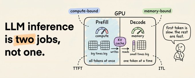![Image](/doc/1507/image/img_d7f93bfa1960.jpg) A first-principles tour of what happens between your prompt and the streamed response: tokenization, embeddings, attention, the prefill/decode split, KV caching, and quantization. You type a prompt. A few hundred milliseconds later, words start streaming back at you one at a time. Feels simple. It isn't. What happens between your keystroke and that first token is one of the most carefully engineered pipelines in modern computing. And the strangest part? The model does two completely different jobs to answer you, with two different bottlenecks, on the same GPU, in the same request. Once you see it, you'll never look at a generate() call the same way again. # The mental model An LLM is a neural network that predicts the next token. Just one token. Then it takes that token, sticks it onto the end of your prompt, and predicts the next one. Then repeats it. That's it. That's the whole loop. The interesting question is: how does it predict that next token, and why does the second token come out much faster than the first? # Step 1: Your text becomes numbers Neural networks don't read English. They read vectors. So the first thing that happens to your prompt is tokenization, which chops your text into pieces and assigns each piece an integer ID. Most modern LLMs use a scheme called Byte Pair Encoding. The idea: start with raw characters, then merge the most common adjacent pairs over and over until you have a vocabulary of ~50,000 chunks. Common words like the get one token. Rare words like unhappiness get split into pieces like un + happi + ness. ``` prompt = "How does inference work?" ids = tokenizer.encode(prompt) # ids -> [2437, 1374, 32278, 670, 30] ``` This step matters more than people realize. Languages that weren't well-represented in the tokenizer's training data get chopped into more pieces, which means more tokens, which means higher cost and slower responses for the same sentence. # Step 2: Each token becomes a vector Each integer ID gets looked up in a giant matrix called the embedding table. If your model has a vocabulary of 50K and a hidden dimension of 4,096, the table has shape [50000, 4096]. Pick a row, get a vector. ``` # embedding_table has shape [vocab_size, hidden_dim] vectors = embedding_table[ids] # shape: [num_tokens, 4096] ``` These vectors aren't random. During training, the model nudged them around so that semantically similar tokens ended up near each other in this 4,096-dimensional space. king and queen are neighbours. python and snake are neighbours along one axis, python and javascript along another. The embedding layer is also where position information gets injected, because attention itself doesn't know which token came first. Modern models use schemes like RoPE that rotate the vectors based on their position in the sequence. 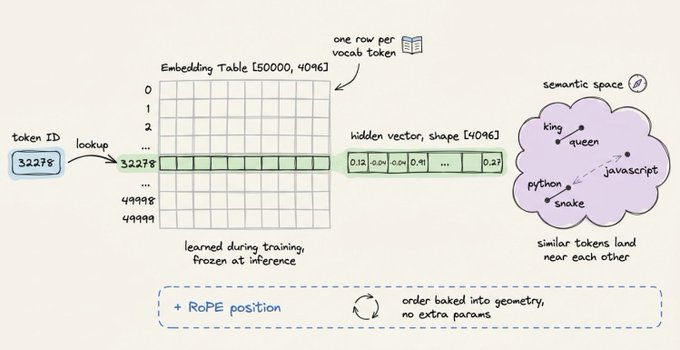![Image](/doc/1507/image/img_60ceda6e46c7.jpg) # Step 3: Layers of attention Now the real work begins. Your sequence of vectors gets fed through a stack of transformer layers, often 32 or more, one after the other. Each layer does roughly the same thing: 1. Mix information across tokens using self-attention. 2. Mix information within each token using a feed-forward network. Self-attention is the part worth understanding deeply. For every token, the layer produces three new vectors by multiplying with three learned weight matrices: ``` # x is the input to this layer, shape [num_tokens, hidden_dim] Q = x @ Wq # queries K = x @ Wk # keys V = x @ Wv # values ``` 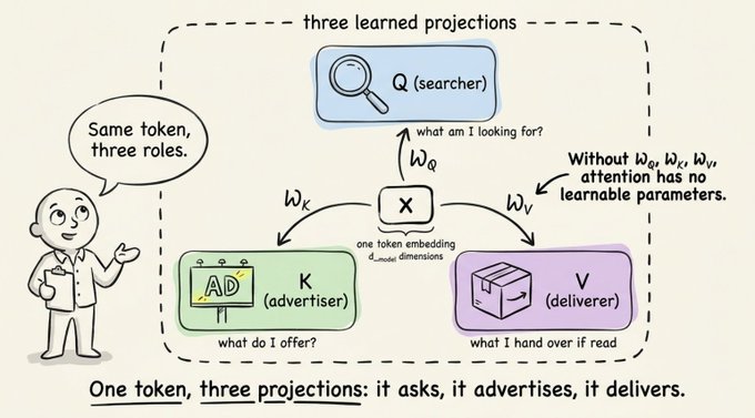![Image](/doc/1507/image/img_98c3ddb893fe.jpg) Now you have three views of every token. The trick: each token uses its query to look at every other token's key, and the strength of the match decides how much of that other token's value to mix in. ``` # scores: how much each token attends to every other token raw = Q @ K.T scaled = raw / sqrt(hidden_dim) # keeps softmax stable weights = softmax(scaled) # one row per token, sums to 1 attention_output = weights @ V ``` Here's a visual representaion of the above process: 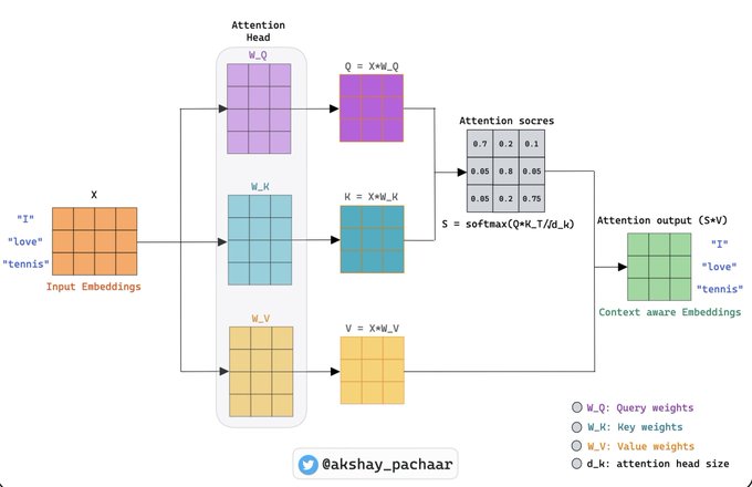![Image](/doc/1507/image/img_16aeed967791.jpg) That's the magic. A token decides what context it needs by looking around and pulling in whatever it finds useful. Stack 32 layers of this and you get a model that can track references across thousands of tokens. After attention, each token's vector goes through a small two-layer feed-forward network that does most of the model's actual "knowing." Attention moves information around. The feed-forward network processes it. # Step 4: Predict the next token After the final layer, the model takes the vector for the last position, projects it back to vocabulary size, and applies softmax to get a probability over every possible next token. Sample from that distribution, and you have your first generated token. Now we hit the interesting part. # The two phases nobody tells you about Generating a 200-token response isn't one task. It's two tasks that look nothing alike under the hood. 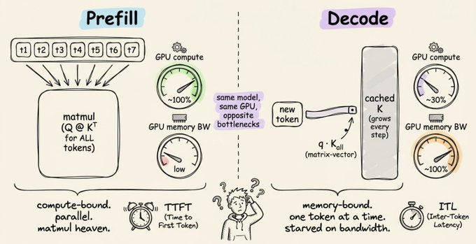![Image](/doc/1507/image/img_3e27412089b6.jpg) ## Phase 1: Prefill When you submit a prompt, the model has to process all of your input tokens before it can generate anything. The good news: it can do this in parallel. Every token's Q, K, and V get computed at the same time. Attention runs as a big matrix-by-matrix multiplication. GPUs love this. Matrix-matrix multiplication is what they were built for. The bottleneck here is raw arithmetic throughput: the GPU is pinned at high utilization, doing math as fast as the silicon allows. The metric for this phase is Time to First Token (TTFT). It's the idle time before the first word shows up on your screen. ``` # Prefill: process the whole prompt in one shot hidden = embed(prompt_tokens) + positions for layer in model.layers: Q, K, V = project(hidden) # for ALL tokens at once hidden = attention(Q, K, V) + hidden hidden = feedforward(hidden) + hidden cache_kv(layer, K, V) # save for later first_token = sample(project_to_vocab(hidden[-1])) ``` ## Phase 2: Decode Once the first token is out, the model switches modes. To generate token 51, it only needs to compute Q, K, and V for that one token. The previous 50 tokens? Their K and V vectors haven't changed. Recomputing them would be wasted work. 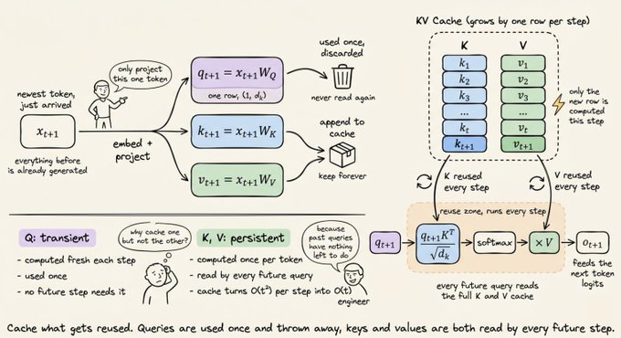![Image](/doc/1507/image/img_551cf5fcc29b.jpg) So the model loops, one token at a time: ``` # Decode: one token per iteration token = first_token steps = 0 while token != STOP and steps < MAX_STEPS: x = embed(token) + position(steps) for layer in model.layers: q, k, v = project(x) K_all, V_all = caches[layer].append(k, v) # cached history + new x = layer.forward(q, K_all, V_all, x) # attention + FFN, residuals token = sample(project_to_vocab(x)) steps += 1 yield token ``` Notice what changed. Instead of multiplying a matrix of queries against a matrix of keys, you're multiplying a single query vector against a matrix of keys. The arithmetic is tiny. But the GPU still has to load every weight matrix from memory and every cached K and V from memory to do that tiny computation. Suddenly the bottleneck flips. The chip has plenty of compute headroom and is just sitting there waiting for memory to deliver the next chunk of data. This is why decode is memory-bound, prefill is compute-bound. Same model, same hardware, totally different performance characteristics. The metric here is Inter-Token Latency (ITL): the gap between consecutive tokens streaming out. Low ITL is what makes a model feel fast. # The KV cache: the optimization that makes this whole thing viable That append_to_cache line above is doing all the heavy lifting. Without it, generating a 1,000-token response would mean recomputing attention for the entire growing sequence at every step. Quadratic complexity and it's painfully slow. With it, you save the K and V matrices once and reuse them forever. Here's the rough shape of what's happening: ``` # One KVCache per transformer layer class KVCache: def __init__(self): self.K = None # all keys seen so far, shape [tokens, dim] self.V = None # all values seen so far, shape [tokens, dim] def append(self, k_new, v_new): if self.K is None: self.K, self.V = k_new, v_new # first token else: self.K = concat([self.K, k_new], axis=token_axis) self.V = concat([self.V, v_new], axis=token_axis) return self.K, self.V # full history so far ``` The speedup is huge. Think 5x or more for long generations. But there's a price: the cache lives in GPU memory, and it grows with every token. Every layer keeps its own K and V tensors. For a 13B model, you're looking at roughly 1 MB per token. A 4K-token context burns through 4 GB of VRAM just on the cache. This is why long contexts feel slow and expensive. It's not the model running out of brainpower. It's the cache running out of room. The fixes are creative: quantize the cache to INT8 or INT4, drop tokens outside a sliding window, share K and V across attention heads (grouped-query attention), or page the cache like an operating system pages memory (PagedAttention, the trick behind vLLM). # Frontier research: shrinking the cache itself Quantization and paging treat the cache as a fixed cost. DeepSeek's V4 series, previewed in late 2025, takes a more aggressive line: redesign attention so the cache is small from the start. Their hybrid scheme combines two compressed attention variants, one sparse, one dense, both operating on a heavily compressed KV stream. At a one-million-token context, V4-Pro reports around 10% of the cache size and 27% of the per-token compute of its predecessor. The takeaway isn't the specific architecture. It's that the KV cache has become the bottleneck the field is now optimizing the model around. When attention itself is being redesigned to minimize the cache, you know the constraint has shifted. Worth a read if you want to see where long-context inference is heading. The full tech report is here: DeepSeek-V4 paper ![Image](/doc/1507/image/img_b110a7b57f2e.jpg) # Quantization: trading bits for speed Training needs precision. Inference doesn't. Most production deployments run in FP16 or BF16 instead of FP32, which halves memory and roughly doubles throughput on Tensor Cores. Aggressive setups go further, quantizing weights to INT8 or even INT4. The math is straightforward. A 7B-parameter model takes: - 28 GB at FP32 - 14 GB at FP16 - 7 GB at INT8 - 3.5 GB at INT4 That last number is why you can run a 7B model on a laptop GPU. Methods like GPTQ and AWQ pick per-channel scaling factors so the lossy compression hurts quality as little as possible. Done well, INT4 can land within a percentage point of the original on most benchmarks. # Putting it all together Here's the full journey of one prompt, end to end: 1. Tokenize. Text becomes integer IDs. 2. Embed. IDs become vectors. Position information gets folded in. 3. Prefill. Every layer runs over every input token in parallel. Compute-bound. The KV cache gets populated. First output token pops out. 4. Decode loop. For each new token: project Q for the new token, attend over the cached K and V, run the feed-forward network, sample. Append the new K and V to the cache. Memory-bound. 5. Detokenize. Token IDs get mapped back to characters and streamed to your screen. Modern serving frameworks like vLLM, TensorRT-LLM, and Text Generation Inference wrap this loop with continuous batching (tokens from multiple users get interleaved on the same GPU step), speculative decoding (a small model drafts tokens, the big model verifies), and clever memory management. That's how a single GPU serves dozens of concurrent users. 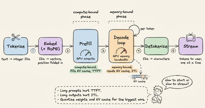![Image](/doc/1507/image/img_a540253dfa1a.jpg) # What this should change about how you think A few practical takeaways once the picture clicks: - Long prompts are expensive in TTFT, long outputs are expensive in ITL. They stress different things. Optimize for the one your users actually feel. - Context length isn't free. Doubling it doesn't just double compute; it bloats the KV cache and starves your batch size. - Quantization is the highest-leverage knob you have. Going FP16 to INT8 often cuts latency in half with negligible quality loss. - GPU utilization can be misleading. A model that pegs the GPU during prefill might be at 30% during decode. The fix isn't more compute; it's faster memory or a smaller cache. The transformer architecture gets all the attention, but inference performance lives or dies on the boring stuff. Memory layout. Cache management. Bit widths. The art is squeezing the most from the hardware you've got. Now when someone tells you their model is slow, you'll know which question to ask first: is it slow to start, or slow to stream? If you liked this article, let me know in the comments. It gives me a signal that I should create more content like this. Thanks for reading! Cheers! :) ## 相关链接 - [Akshay](https://x.com/akshay_pachaar) - [@akshay_pachaar](https://x.com/akshay_pachaar) - [1.7K](https://x.com/akshay_pachaar/status/2050941458614751327/analytics) - [DeepSeek-V4 paper](https://huggingface.co/deepseek-ai/DeepSeek-V4-Pro/blob/main/DeepSeek_V4.pdf) - [vLLM](https://github.com/vllm-project/vllm) - [TensorRT-LLM](https://github.com/NVIDIA/TensorRT-LLM) - [Upgrade to Premium](https://x.com/i/premium_sign_up) - [10:12 PM · May 3, 2026](https://x.com/akshay_pachaar/status/2050941458614751327) - [1,716 Views](https://x.com/akshay_pachaar/status/2050941458614751327/analytics) --- *导出时间: 2026/5/3 22:41:45* --- ## 中文翻译 # LLM 推理是如何工作的 **作者**: Akshay **日期**: 2026-05-03T14:12:03.000Z **来源**: [https://x.com/akshay_pachaar/status/2050941458614751327](https://x.com/akshay_pachaar/status/2050941458614751327) --- ![Image](/doc/1507/image/img_d7f93bfa1960.jpg) 这是一次基于第一性原理的探索，带你了解在你的提示词和流式响应之间发生了什么：分词、嵌入、注意力机制、预填充/解码分离、KV 缓存以及量化。你输入一个提示词。几百毫秒后，文字开始一个接一个地流回来。感觉很简单。其实不然。在你的按键按下和第一个 token 出现之间发生的事情，是现代计算中经过最精心设计的流程之一。最奇怪的部分是什么？为了回答你，模型在同一个 GPU 上处理同一个请求时，要做两种完全不同的工作，并且受限于两种不同的瓶颈。一旦你看清了这一点，你以后再看待 `generate()` 调用时就会不一样了。 # 思维模型 LLM 是一个预测下一个 token 的神经网络。仅仅是一个 token。然后它获取那个 token，将其附加到你的提示词末尾，并预测下一个。然后重复。就是这样。这就是整个循环。有趣的问题是：它是如何预测下一个 token 的，以及为什么第二个 token 的输出速度比第一个快得多？ # 第 1 步：你的文本变成了数字神经网络不读英语。它们读向量。所以你的提示词遇到的第一件事就是分词，它把你的文本切碎并给每一块分配一个整数 ID。大多数现代 LLM 使用一种称为字节对编码的方案。其思想是：从原始字符开始，然后不断合并最常见的相邻对，直到你有一个大约 50,000 个块的词汇表。像 "the" 这样的常用词得到一个 token。像 "unhappiness" 这样的罕见词被分割成 "un" + "happi" + "ness" 这样的块。 ``` prompt = "How does inference work?" ids = tokenizer.encode(prompt) # ids -> [2437, 1374, 32278, 670, 30] ``` 这一步的重要性比人们意识到的要大。在分词器训练数据中代表性不足的语言会被切碎成更多块，这意味着更多的 token，这意味着对于相同的句子，成本更高，响应更慢。 # 第 2 步：每个 token 变成一个向量每个整数 ID 都在一个叫做嵌入表的巨大矩阵中被查找。如果你的模型有 50K 的词汇量和 4,096 的隐藏维度，表的形状就是 [50000, 4096]。选一行，得到一个向量。 ``` # embedding_table 的形状是 [vocab_size, hidden_dim] vectors = embedding_table[ids] # 形状: [num_tokens, 4096] ``` 这些向量不是随机的。在训练期间，模型调整了它们，使得语义相似的 token 在这个 4,096 维的空间中最终彼此靠近。"king" 和 "queen" 是邻居。Python 和 "snake" 沿一个轴是邻居，Python 和 "javascript" 沿另一个轴是邻居。嵌入层也是注入位置信息的地方，因为注意力机制本身不知道哪个 token 先出现。现代模型使用像 RoPE 这样的方案，根据向量在序列中的位置旋转它们。 ![Image](/doc/1507/image/img_60ceda6e46c7.jpg) # 第 3 步：注意力的层级现在真正的工作开始了。你的向量序列被送入一堆 transformer 层，通常有 32 层或更多，一层接一层。每一层大致做同样的事情： 1. 使用自注意力在 token 之间混合信息。 2. 使用前馈网络在每个 token 内部混合信息。自注意力是值得深入理解的部分。对于每个 token，该层通过乘以三个学习的权重矩阵产生三个新向量： ``` # x 是该层的输入，形状 [num_tokens, hidden_dim] Q = x @ Wq # queries K = x @ Wk # keys V = x @ Wv # values ``` ![Image](/doc/1507/image/img_98c3ddb893fe.jpg) 现在你有了每个 token 的三种视图。诀窍在于：每个 token 使用它的查询去查看每个其他 token 的键，匹配的强度决定了混合多少该其他 token 的值。 ``` # scores: 每个 token 关注多少每个其他 token raw = Q @ K.T scaled = raw / sqrt(hidden_dim) # 保持 softmax 稳定 weights = softmax(scaled) # 每个 token 一行，总和为 1 attention_output = weights @ V ``` 这是上述过程的可视化表示： ![Image](/doc/1507/image/img_16aeed967791.jpg) 这就是魔法所在。一个 token 通过四处观察并引入它发现的有用内容来决定它需要什么上下文。堆叠 32 层这样的结构，你就会得到一个可以跨数千个 token 追踪引用的模型。在注意力之后，每个 token 的向量通过一个小的两层前馈网络，该网络完成了模型大部分实际的“认知”工作。注意力负责移动信息。前馈网络负责处理信息。 # 第 4 步：预测下一个 token 在最后一层之后，模型取最后位置的向量，将其投影回词汇表大小，并应用 softmax 以获得每个可能的下一个 token 的概率。从该分布中采样，你就得到了你的第一个生成的 token。现在我们要到了有趣的部分。 # 没人告诉你的两个阶段生成一个 200 token 的响应不是一项任务。它是两项在内部看起来完全不同的任务。 ![Image](/doc/1507/image/img_3e27412089b6.jpg) ## 阶段 1：预填充当你提交提示词时，模型必须处理所有的输入 token 才能生成任何东西。好消息是：它可以并行地做这件事。每个 token 的 Q、K 和 V 同时被计算。注意力作为一个大的矩阵对矩阵乘法运行。 GPU 喜欢这个。矩阵-矩阵乘法就是它们的构建目的。这里的瓶颈是原始算力吞吐量：GPU 被固定在高利用率，以硅允许的速度尽可能快地做数学运算。这个阶段的指标是首字延迟。这是第一个词出现在你的屏幕之前的空闲时间。 ``` # Prefill: 一次性处理整个提示词 hidden = embed(prompt_tokens) + positions for layer in model.layers: Q, K, V = project(hidden) # 立即为所有 token 计算 hidden = attention(Q, K, V) + hidden hidden = feedforward(hidden) + hidden cache_kv(layer, K, V) # 留作后用 first_token = sample(project_to_vocab(hidden[-1])) ``` ## 阶段 2：解码一旦第一个 token 出来，模型就切换模式。为了生成第 51 个 token，它只需要计算那一个 token 的 Q、K 和 V。前 50 个 token 呢？它们的 K 和 V 向量没有改变。重新计算它们将是浪费工作。 ![Image](/doc/1507/image/img_551cf5fcc29b.jpg) 所以模型循环，一次一个 token： ``` # Decode: 每次迭代一个 token token = first_token steps = 0 while token != STOP and steps < MAX_STEPS: x = embed(token) + position(steps) for layer in model.layers: q, k, v = project(x) K_all, V_all = caches[layer].append(k, v) # 缓存的历史记录 + 新的 x = layer.forward(q, K_all, V_all, x) # attention + FFN, residuals token = sample(project_to_vocab(x)) steps += 1 yield token ``` 注意发生了什么变化。你不再是用查询矩阵乘以键矩阵，而是用单个查询向量乘以键矩阵。计算量微乎其微。但 GPU 仍然必须从内存中加载每个权重矩阵，并从内存中加载每个缓存的 K 和 V 来做那个微小的计算。突然间瓶颈翻转了。芯片有大量的计算余量，只是坐在那里等待内存传递下一块数据。这就是为什么解码是内存受限的，而预填充是计算受限的。相同的模型，相同的硬件，完全不同的性能特征。这里的指标是 Token 间延迟：流出的连续 token 之间的间隔。低 ITL 是让模型感觉快的原因。 # KV 缓存：让这一切可行的优化上面的 `append_to_cache` 行正在做所有繁重的工作。如果没有它，生成一个 1,000 token 的响应将意味着在每一步重新计算整个增长序列的注意力。二次方复杂度，而且慢得痛苦。有了它，你只需保存 K 和 V 矩阵一次并永远重用它们。这里是大致发生的事情的形状： ``` # 每个 transformer 层一个 KVCache class KVCache: def __init__(self): self.K = None # 目前为止看到的所有键，形状 [tokens, dim] self.V = None # 目前为止看到的所有值，形状 [tokens, dim] def append(self, k_new, v_new): if self.K is None: self.K, self.V = k_new, v_new # 第一个 token else: self.K = concat([self.K, k_new], axis=token_axis) self.V = concat([self.V, v_new], axis=token_axis) return self.K, self.V # 目前的完整历史 ``` 加速是巨大的。对于长生成，可以想到 5 倍或更多。但有一个代价：缓存存在于 GPU 内存中，并且随着每个 token 的增长。每一层都保留自己的 K 和 V 张量。对于一个 13B 的模型，每个 token 大约需要 1 MB。一个 4K token 的上下文仅缓存就要消耗 4 GB 的 VRAM。这就是为什么长上下文感觉缓慢且昂贵。不是模型脑子不够用。是缓存空间不够了。修复方案很有创意：将缓存量化为 INT8 或 INT4，丢弃滑动窗口之外的 token，在注意力头之间共享 K 和 V（分组查询注意力），或者像操作系统分页内存一样对缓存进行分页。 # 前沿研究：缩小缓存本身量化和分页将缓存视为固定成本。DeepSeek 的 V4 系列，于 2025 年底预览，采取了一种更激进的路线：重新设计注意力，使缓存从一开始就很小。他们的混合方案结合了两种压缩注意力的变体，一种是稀疏的，一种是密集的，都在重度压缩的 KV 流上运行。在一百万 token 的上下文中，V4-Pro 报告的缓存大小约为其前身的 10%，每 token 计算量为 27%。结论不在于特定的架构。而在于 KV 缓存已成为瓶颈，该领域现在正围绕优化缓存来设计模型。当注意力本身被重新设计以最小化缓存时，你就知道约束已经转移了。如果你想看看长上下文推理的发展方向，值得一读。完整的技术报告在这里：DeepSeek-V4 论文 ![Image](/doc/1507/image/img_b110a7b57f2e.jpg) # 量化：用比特换速度训练需要精度。推理不需要。大多数生产部署在 FP16 或 BF16 而不是 FP32 下运行，这使内存减半，并在 Tensor Core 上大约使吞吐量翻倍。激进的设置更进一步，将权重量化为 INT8 甚至 INT4。数学计算很简单。一个 7B 参数的模型需要： - FP32 下 28 GB - FP16 下 14 GB - INT8 下 7 GB - INT4 下 3.5 GB 最后一个数字就是为什么你可以在笔记本电脑 GPU 上运行 7B 模型。像 GPTQ 和 AWQ 这样的方法选择每通道缩放因子，以便有损压缩尽可能少地损害质量。如果做得好，在大多数基准测试中 INT4 可以落在原始模型的一个百分点内。 # 把所有东西放在一起这是一个提示词的完整旅程，端到端： 1. 分词。文本变成整数 ID。 2. 嵌入。ID 变成向量。位置信息被折叠进去。 3. 预填充。每一层并行地处理每个输入 token。计算受限。KV 缓存被填充。第一个输出 token 弹出。 4. 解码循环。对于每个新 token：为新 token 投影 Q，对缓存的 K 和 V 进行注意力计算，运行前馈网络，采样。将新的 K 和 V 附加到缓存。内存受限。 5. 解分词。Token ID 被映射回字符并流式传输到你的屏幕。现代服务框架，如 vLLM、TensorRT-LLM 和 Text Generation Inference，用连续批处理（来自多个用户的 token 在同一个 GPU 步骤中交错）、投机解码（一个小模型起草 token，大模型验证）和巧妙的内存管理来包装这个循环。这就是单个 GPU 为几十个并发用户服务的原因。 ![Image](/doc/1507/image/img_a540253dfa1a.jpg) # 这应该如何改变你的思考方式一旦图景清晰，一些实用的要点： - 长提示词在 TTFT 方面很昂贵，长输出在 ITL 方面很昂贵。它们给不同的部分带来压力。针对你的用户实际感受到的那个进行优化。 - 上下文长度不是免费的。将其翻倍不仅会使计算翻倍；它还会膨胀 KV 缓存并挤占你的批处理大小。 - 量化是你拥有的最高杠杆的旋钮。从 FP16 到 INT8 通常会将延迟减半，而质量损失可以忽略不计。 - GPU 利用率可能会产生误导。一个在预填充期间占用 GPU 的模型在解码期间可能只有 30%。修复方法不是更多的计算；而是更快的内存或更小的缓存。 Transformer 架构获得了所有的关注，但推理性能的死活取决于那些无聊的东西。内存布局。缓存管理。位宽。艺术在于从你拥有的硬件中挤出最多的性能。现在，当有人告诉你他们的模型很慢时，你会知道该先问哪个问题：是启动慢，还是流式传输慢？如果你喜欢这篇文章，请在评论中告诉我。这给了我一个信号，我应该创建更多这样的内容。感谢阅读！干杯！ :) ## 相关链接 - [Akshay](https://x.com/akshay_pachaar) - [@akshay_pachaar](https://x.com/akshay_pachaar) - [1.7K](https://x.com/akshay_pachaar/status/2050941458614751327/analytics) - [DeepSeek-V4 paper](https://huggingface.co/deepseek-ai/DeepSeek-V4-Pro/blob/main/DeepSeek_V4.pdf) - [vLLM](https://github.com/vllm-project/vllm) - [TensorRT-LLM](https://github.com/NVIDIA/TensorRT-LLM) - [Upgrade to Premium](https://x.com/i/premium_sign_up) - [10:12 PM · May 3, 2026](https://x.com/akshay_pachaar/status/2050941458614751327) - [1,716 Views](https://x.com/akshay_pachaar/status/2050941458614751327/analytics) --- *导出时间: 2026/5/3 22:41:45*

🔗 相关文档